This book contains both practical guides on exploring missing data, as well as some of the deeper details of how naniar works to help you better explore your missing data. A large component of this book are the exercises that accompany each section in each chapter.
In this chapter we discuss whether imputation is appropriate, and the features of good and bad imputations. You will learn how to evaluate imputed values by using visualisations to assess their summary features: the mean/median, scale, and spread.
13.1 What makes a good imputation
Imputing missing values needs to be done with care - you want to avoid imputing unlikely values like mid winter temperatures into the middle of summer, giving pigs a wing span measurement, or heavy rainfall into a known drought.
13.2 When to impute
Not everything can be solved with imputation. If you don’t already have the information, sometimes it is not appropriate to impute variables like, age, race, sex and gender without first confirming known facts about your population. Sometimes this means talking to the person who collected or curated the data to understand the population studied. You might learn some variables remain fixed over time, and so can be perfectly imputed. Other times, we might not know, so leaving the values as missing might be the most appropriate action. Imputation isn’t always the answer.
Another consideration for imputation is when there is simply too much missing data. For example, if you have a variable with 50% of the values missing, imputation might not be appropriate unless you have a very strong modelling case. For example, you know all the ages were not recorded for every person, but were the same for each person, so you can impute perfectly. When there are missing values in the outcome variable (the “Y”, the Dependent Variable, DV, it has many names!), it is generally not a good idea to impute data for these values. The reason is that you are effectively using the data twice.
[TODO: add a small simulation on this]
[TODO: add caveats around Bayesian/likelihood simulation approaches]
13.3 Understanding the good by understanding the bad
To understand good imputation, it is useful to understand bad imputations. One particularly bad imputation is mean imputation, which takes the mean of complete values as the imputed value.
For example, in a dataframe with 5 values and one missing, we calculate the mean from complete observations using na.rm = TRUE, and use this to impute the missing values. The steps are shown here:
df <-tibble(x =c(1, 4, 9, 16, NA, 36))df
# A tibble: 6 × 1
      x
  <dbl>
1     1
2     4
3     9
4    16
5    NA
6    36
mean(df$x, na.rm =TRUE)
[1] 13.2
df[is.na(df)] <-mean(df$x, na.rm =TRUE)df
# A tibble: 6 × 1
      x
  <dbl>
1   1
2   4
3   9
4  16
5  13.2
6  36
13.3.1 Demonstrating mean imputation
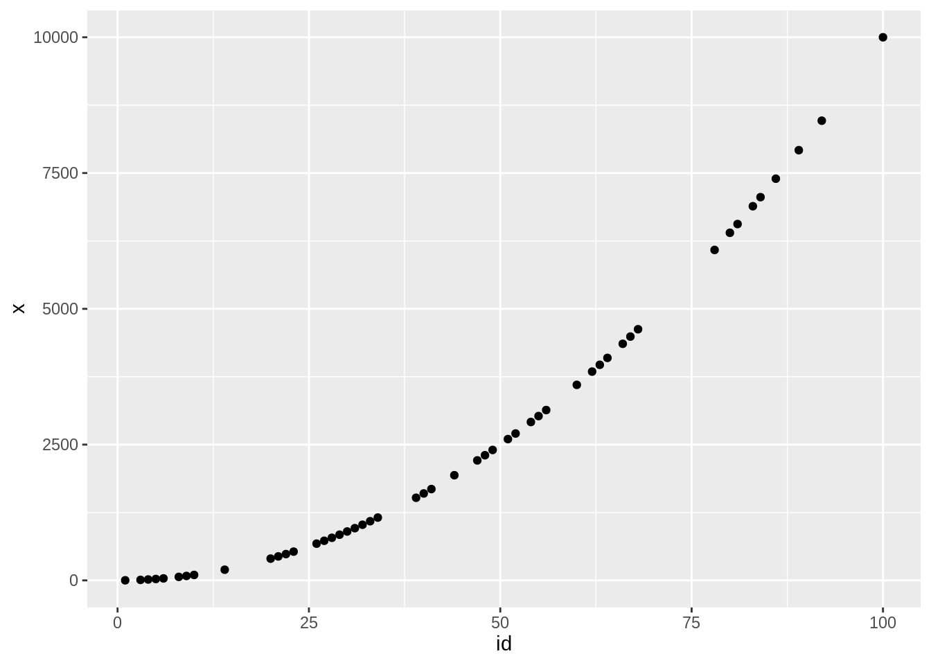
This is generally a terribly idea. For example, imagine we had data like this, with missing values:
The mean does not respect the underlying process of the data. Visualisation is a very key tool here to explore and demonstrate this pattern.
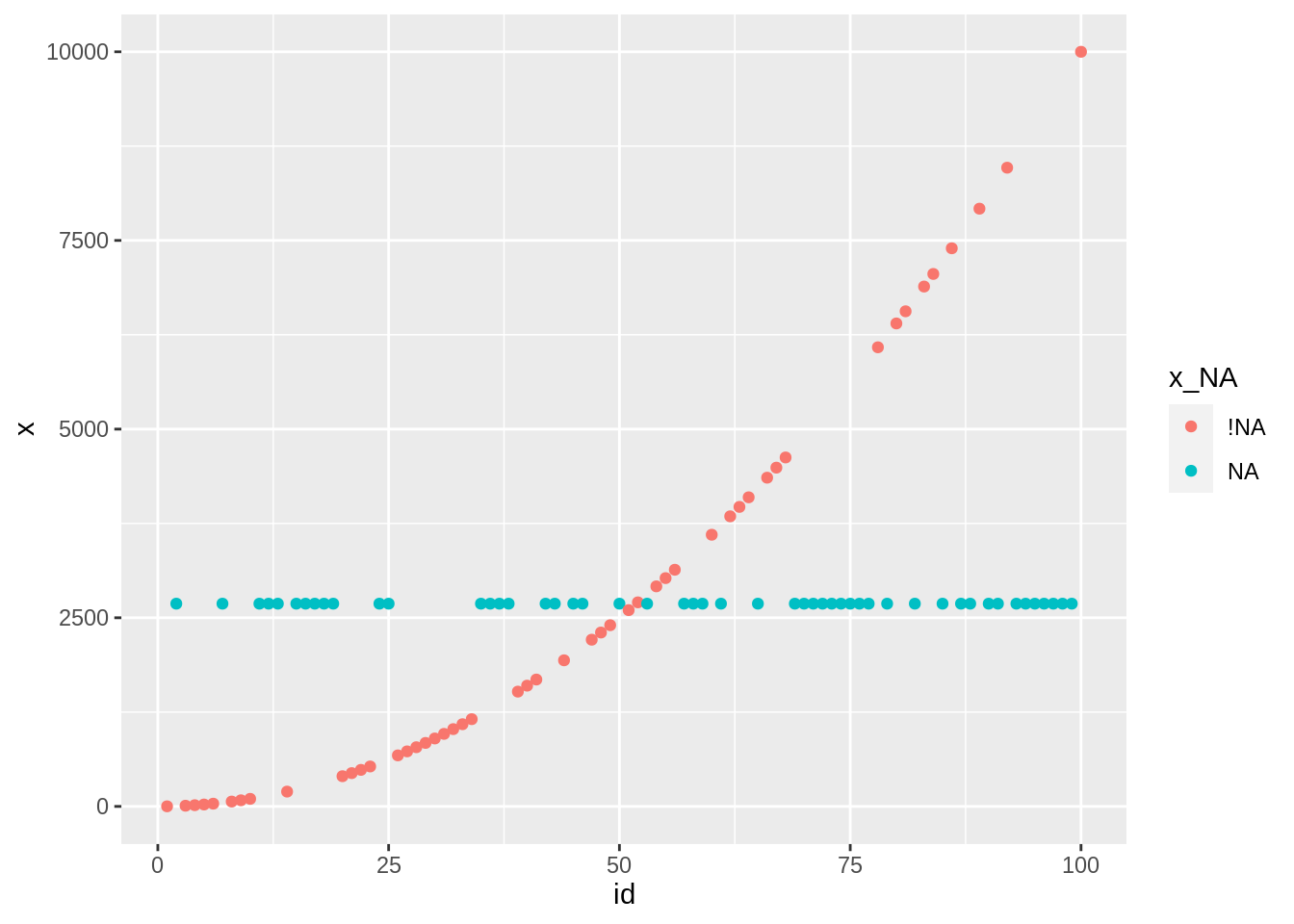
13.3.2 Explore bad imputations: The mean
To examine these bad imputations, we use the impute_mean function from the naniar package. Similar to impute_below used in the previous chapter, we can use across and friends with impute_mean. So it can work on a vector, on variables based on some condition like are they numeric, for specified variables, or for all variables.
13.3.3 Tracking missing values
To visualise imputations we use the same process as for impute_below:
# A tibble: 153 × 9
   Ozone Solar.R  Wind  Temp Month   Day Ozone_NA Solar.R_NA any_missing
   <dbl>   <dbl> <dbl> <dbl> <dbl> <dbl> <fct>    <fct>      <chr>
 1  41      190    7.4    67     5     1 !NA      !NA        Not Missing
 2  36      118    8      72     5     2 !NA      !NA        Not Missing
 3  12      149   12.6    74     5     3 !NA      !NA        Not Missing
 4  18      313   11.5    62     5     4 !NA      !NA        Not Missing
 5  42.1    186.  14.3    56     5     5 NA       NA         Missing
 6  28      186.  14.9    66     5     6 !NA      NA         Missing
 7  23      299    8.6    65     5     7 !NA      !NA        Not Missing
 8  19       99   13.8    59     5     8 !NA      !NA        Not Missing
 9   8       19   20.1    61     5     9 !NA      !NA        Not Missing
10  42.1    194    8.6    69     5    10 NA       !NA        Missing
# … with 143 more rows
We first create nabular data to track missing values. Then, we do our imputations. Then, we add a label to identify cases with missing observations using add_label_shadow(). One thing to have up your sleeve it only_miss option, which binds only columns with missing values. This makes the data bit smaller and easier to handle.
Now that we know a way to impute our data, let’s explore it. We can explore the imputed values in the same way we did for the previous lesson. But this time our intention is different, and we want to consider evaluating imputations by looking for changes in the mean, the spread, and the scale.
[TODO **A small figure/plot that clearly shows what we mean by mean, spread, scale]**
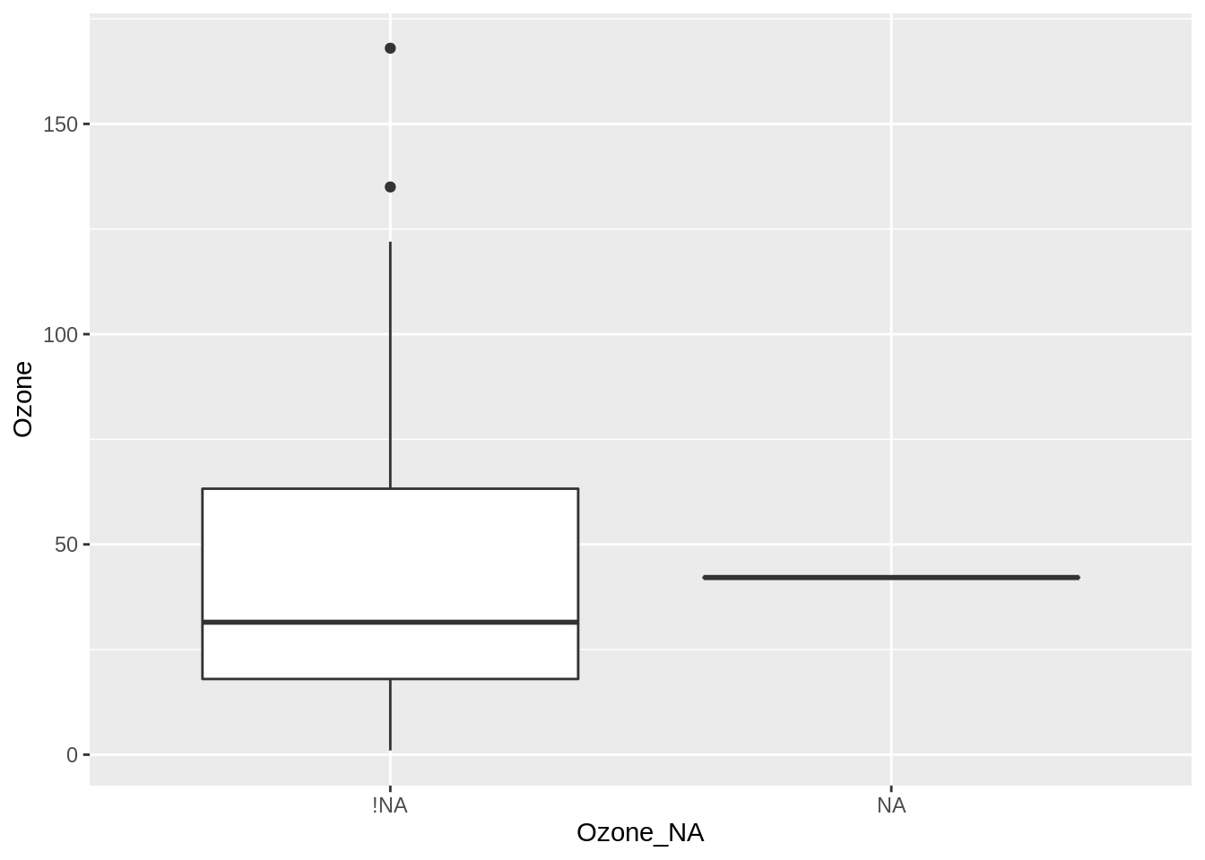
13.3.4 Using a boxplot to explore how the mean changes
We can evaluate changes in the mean or median using a boxplot. We put the missingness of ozone, ozone_NA, on the x axis, and the values of ozone on the y axis, and use geom_boxplot.
From this visualisation, we learn the median value is similar in each group, but the median is lower for the not missing group. The take away message is the mean isn’t changing. This is good, but there is more than one feature to explore!
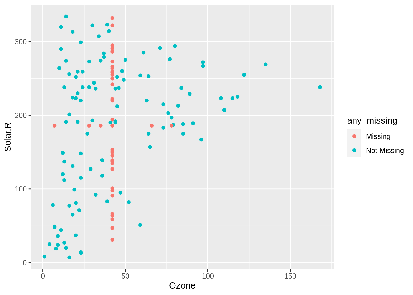
13.4 Using a scatterplot to Explore how spread changes with imputation
The spread of imputations can be explored using a scatter plot. We plot our airquality imputed with the mean, with Ozone and solar radiation on the x and y axis, and colouring according to missingness, any_missing.
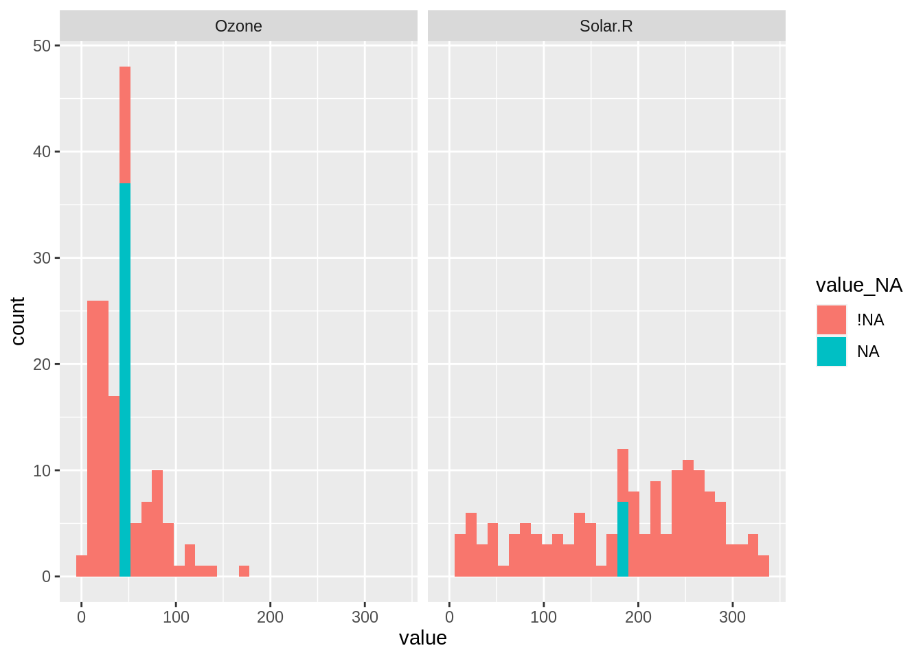
To make it easier to explore many variables, we use the shadow_long function to return nabular data in long format. This is similar to pivot_longer, but with our nabular data.
Here, we enter in our data, followed by the variables that we want to focus on - in this case, Ozone and Solar.R. This returns to us data with the columns variable, value, and the shadow columns, variable_NA and value_NA.
13.4.2 Exploring imputations for many variables
We can then use this in a ggplot, placing value in the x axis, and filling by the missingness of the value, value_NA, and then using geom_histogram, facetting by variable.