15  Assessing inference from imputation

This book contains both practical guides on exploring missing data, as well as some of the deeper details of how naniar works to help you better explore your missing data. A large component of this book are the exercises that accompany each section in each chapter.

library(naniar)
library(tidyverse)
── Attaching packages ─────────────────────────────────────── tidyverse 1.3.1 ──
✔ ggplot2 3.3.6     ✔ purrr   0.3.4
✔ tibble  3.1.7     ✔ dplyr   1.0.9
✔ tidyr   1.2.0     ✔ stringr 1.4.0
✔ readr   2.1.2     ✔ forcats 0.5.1
── Conflicts ────────────────────────────────────────── tidyverse_conflicts() ──
✖ dplyr::filter() masks stats::filter()
✖ dplyr::lag()    masks stats::lag()
library(simputation)

Attaching package: 'simputation'
The following object is masked from 'package:naniar':

    impute_median

In this chapter we discuss methods for assessing model inference across differently imputed datasets. Let’s step back, and think about why we are imputing data in the first place. Our goal in performing imputations is to perform an analysis in a way that the missing values do not unfairly bias subsequent inference, or predictions that we make.

15.1 Exploring parameters of one model

[TODO: update from airquality dataset, it is getting a bit tired]

Let’s fit a model to the airquality dataset using a linear model, predicting temperature, using ozone, solar radiation, wind, month and day.

lm(Temp ~ Ozone + Solar.R + Wind + Month + Day, data = airquality)

Call:
lm(formula = Temp ~ Ozone + Solar.R + Wind + Month + Day, data = airquality)

Coefficients:
(Intercept)        Ozone      Solar.R         Wind        Month          Day  
   57.25183      0.16528      0.01082     -0.17433      2.04246     -0.08919  

We are going to fit this model using two methods:

  1. Complete case analysis, where we remove all rows that contain a missing value
  2. Imputing data using the linear model imputation from the last lesson.

Using the complete cases provides a nice baseline for comparison, as this removes all missing values, so it is sort of like comparing your model to “doing nothing”. Except that it is worse than doing nothing - since you are removing data! You might be able to imagine a few different outcomes of this process:

  • The outputs are basically the same, in which case, using the data with imputed values is better from a statistics standpoint, so you may as well use them.
  • The imputed data does much better than complete cases, in which case, use the imputed data.
  • The imputed data does worse than complete cases - which which case, you might want to check your imputed model for errors, or perhaps there are some bias in your data.

15.2 Combining the datasets together

There are three steps to comparing our data.

First, we perform the complete case analysis, using na.omit(), and converting the data into nabular form.

#1.  Complete cases
aq_cc <-   airquality %>%
  na.omit() %>%
  nabular() %>% 
  add_label_shadow()

Second, we impute the data according to a linear model

#2. Imputation using the imputed data from the last lesson
aq_imp_lm <- airquality %>% 
  nabular() %>%
  add_label_shadow() %>%
  as.data.frame() %>% 
  impute_lm(Ozone ~ Temp + Wind + Month + Day) %>%
  impute_lm(Solar.R ~ Temp + Wind + Month + Day)  %>% 
  as_tibble()

Finally, we combine the different datasets together with bind_rows(). Note the extra column, imp_model, which helps us identify data from the model used.

# 3. Bind the models together
bound_models <- bind_rows(cc = aq_cc,
                          imp_lm = aq_imp_lm,
                          .id = "imp_model")

This prepares us for fitting our new models, so we can summarise and compare differences in the data.

The bound models have a column imp_model, then the columns from airquality, and our shadow variables and any_missing.

head(bound_models)
# A tibble: 6 × 14
  imp_model Ozone Solar.R  Wind  Temp Month   Day Ozone_NA Solar.R_NA Wind_NA
  <chr>     <dbl>   <dbl> <dbl> <int> <int> <int> <fct>    <fct>      <fct>  
1 cc           41     190   7.4    67     5     1 !NA      !NA        !NA    
2 cc           36     118   8      72     5     2 !NA      !NA        !NA    
3 cc           12     149  12.6    74     5     3 !NA      !NA        !NA    
4 cc           18     313  11.5    62     5     4 !NA      !NA        !NA    
5 cc           23     299   8.6    65     5     7 !NA      !NA        !NA    
6 cc           19      99  13.8    59     5     8 !NA      !NA        !NA    
# … with 4 more variables: Temp_NA <fct>, Month_NA <fct>, Day_NA <fct>,
#   any_missing <chr>
tail(bound_models)
# A tibble: 6 × 14
  imp_model Ozone Solar.R  Wind  Temp Month   Day Ozone_NA Solar.R_NA Wind_NA
  <chr>     <dbl>   <dbl> <dbl> <int> <int> <int> <fct>    <fct>      <fct>  
1 imp_lm     14        20  16.6    63     9    25 !NA      !NA        !NA    
2 imp_lm     30       193   6.9    70     9    26 !NA      !NA        !NA    
3 imp_lm     26.9     145  13.2    77     9    27 NA       !NA        !NA    
4 imp_lm     14       191  14.3    75     9    28 !NA      !NA        !NA    
5 imp_lm     18       131   8      76     9    29 !NA      !NA        !NA    
6 imp_lm     20       223  11.5    68     9    30 !NA      !NA        !NA    
# … with 4 more variables: Temp_NA <fct>, Month_NA <fct>, Day_NA <fct>,
#   any_missing <chr>

15.3 Exploring the models

Now that we’ve got our data in the right format, we fit a linear model to each of the datasets. We use the “many models” approach, covered in detail in the R for data science book by Hadley Wickham and Garrett Grolemund.

This involves some functions that we haven’t seen before. Let’s unpack what’s happening below. First we group by the imputation model, then nest the data. This collapses, or nests, the data down into a neat format where each row is one of our datasets.

bound_models %>% 
  group_by(imp_model) %>%
  nest()
# A tibble: 2 × 2
# Groups:   imp_model [2]
  imp_model data               
  <chr>     <list>             
1 cc        <tibble [111 × 13]>
2 imp_lm    <tibble [153 × 13]>

This allows us to create linear models on each row of the data, using mutate, and a special function, map. This tells the function we are applying to look at the data and then fit the linear model to each of the datasets in the data column.

bound_models %>% 
  group_by(imp_model) %>%
  nest() %>%
  mutate(mod = map(data, 
                   ~lm(Temp ~ Ozone + Solar.R + Wind + Day + Month, 
                       data = .)))
# A tibble: 2 × 3
# Groups:   imp_model [2]
  imp_model data                mod   
  <chr>     <list>              <list>
1 cc        <tibble [111 × 13]> <lm>  
2 imp_lm    <tibble [153 × 13]> <lm>  

Then we then fit the model and create separate columns for residuals, predictions, and coefficients, using the tidy function from broom, to provide nicely formatted coefficients from our linear model.

model_summary <- bound_models %>% 
  group_by(imp_model) %>%
  nest() %>%
  mutate(mod = map(data, 
                   ~lm(Temp ~ Ozone + Solar.R + Wind + Day + Month, 
                       data = .)),
         res = map(mod, residuals),
         pred = map(mod, predict),
         tidy = map(mod, broom::tidy))

model_summary
# A tibble: 2 × 6
# Groups:   imp_model [2]
  imp_model data                mod    res         pred        tidy            
  <chr>     <list>              <list> <list>      <list>      <list>          
1 cc        <tibble [111 × 13]> <lm>   <dbl [111]> <dbl [111]> <tibble [6 × 5]>
2 imp_lm    <tibble [153 × 13]> <lm>   <dbl [153]> <dbl [153]> <tibble [6 × 5]>

Our data, model_summary, has the columns imp_model, and data, and columns with our fitted linear model (mod), residuals (res), predictions (pred), and tidy coefficients (tidy).

model_summary forms the building block for the next steps in our analysis, where we are going to look at the coefficients, the residuals, and the predictions.

This is just one way to fit these kinds of models - there are many other ways, and it might not work for all types of models, but this many models approach can be convenient!

15.4 Exploring coefficients of multiple models

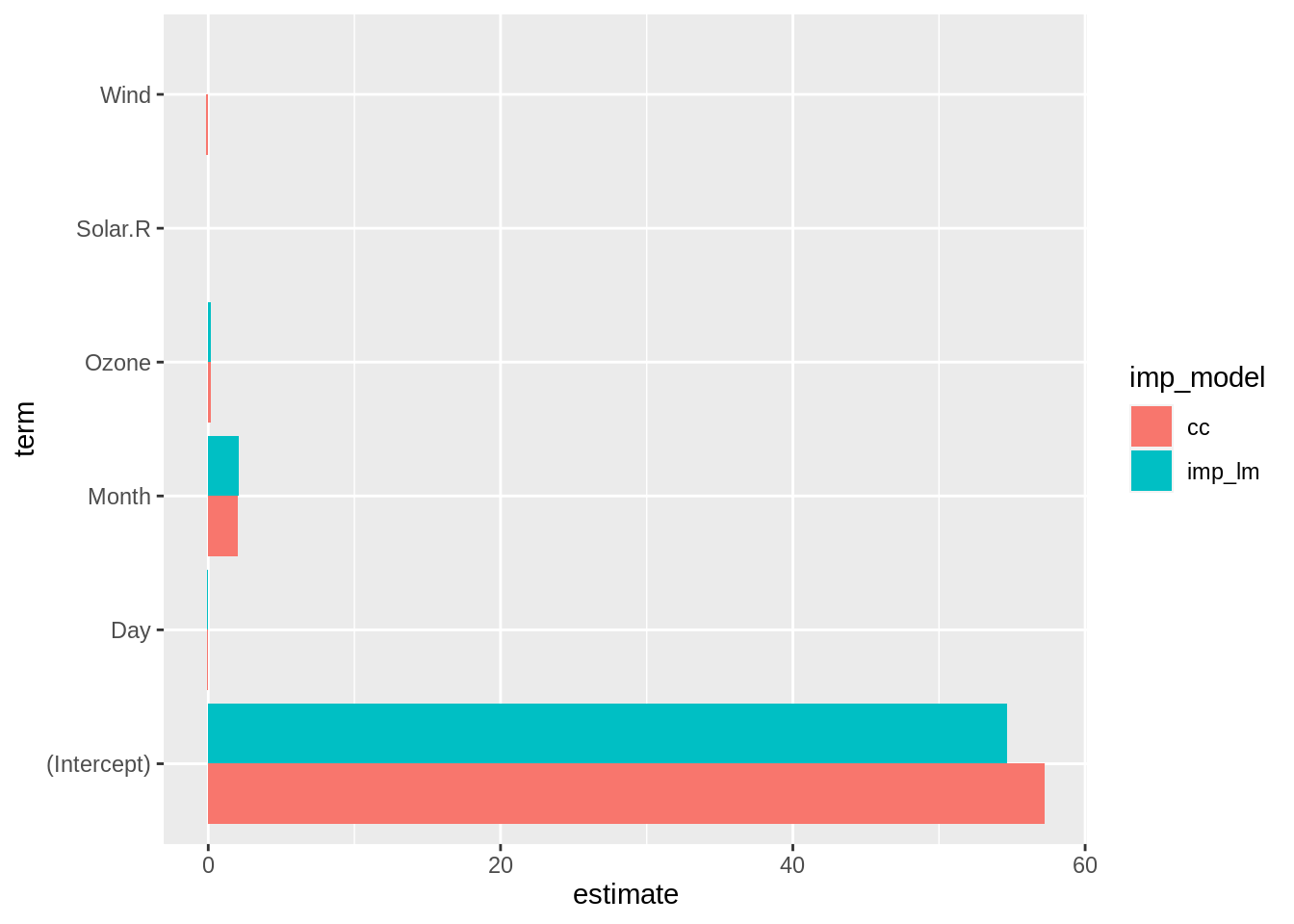
We explore coefficients by selecting the imputation model and the tidy column and unnesting:

model_summary_coefs <- model_summary %>% 
  select(imp_model,
         tidy) %>%
  unnest(cols = c(tidy))

model_summary_coefs
# A tibble: 12 × 6
# Groups:   imp_model [2]
   imp_model term        estimate std.error statistic  p.value
   <chr>     <chr>          <dbl>     <dbl>     <dbl>    <dbl>
 1 cc        (Intercept) 57.3       4.50      12.7    5.52e-23
 2 cc        Ozone        0.165     0.0239     6.92   3.66e-10
 3 cc        Solar.R      0.0108    0.00699    1.55   1.24e- 1
 4 cc        Wind        -0.174     0.212     -0.821  4.13e- 1
 5 cc        Day         -0.0892    0.0677    -1.32   1.91e- 1
 6 cc        Month        2.04      0.409      4.99   2.42e- 6
 7 imp_lm    (Intercept) 54.7       3.59      15.2    5.21e-32
 8 imp_lm    Ozone        0.196     0.0205     9.53   4.52e-17
 9 imp_lm    Solar.R      0.0102    0.00577    1.76   7.97e- 2
10 imp_lm    Wind        -0.00642   0.172     -0.0374 9.70e- 1
11 imp_lm    Day         -0.112     0.0538    -2.08   3.92e- 2
12 imp_lm    Month        2.11      0.340      6.21   5.09e- 9

We now see the estimates of the impact of Ozone on temperature. To best understand this we can plot these estimates for each model like so:

ggplot(model_summary_coefs,
       aes(x = estimate,
           y = term,
           fill = imp_model)) + 
  geom_col(position = "dodge")

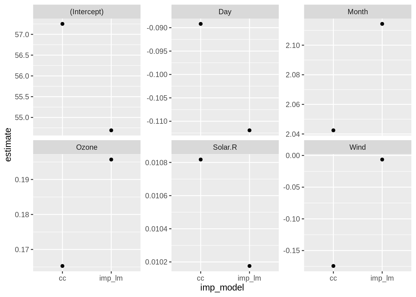
Plotting these, we see that the estimates are pretty much the same for both, with the intercept being slightly lower for the imputed model, and higher for the complete cases. However, we can probably get a slightly more nuanced view of this by looking at these variables on their own scale:

ggplot(model_summary_coefs,
       aes(x = imp_model,
           y = estimate)) + 
  geom_point() + 
  facet_wrap(~term, scales = "free_y")

These look like big differences for all of these - but this is intentional, as we have let the y axis be freely varying. These values in this case look to be not very different in a meaningful way for this data, but it is an important step to take for any dataset.

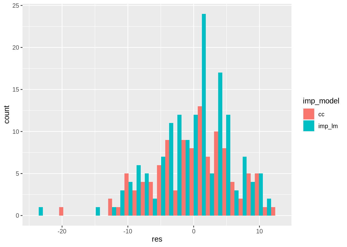
15.5 Exploring residuals of multiple models

Let’s explore the residuals by selecting the imp model and residuals, and then unnesting the data. We can then create a histogram, using position = "dodge" to put residuals for each model next to each other.

model_summary %>% 
  select(imp_model,
         res) %>%
  unnest(cols = c(res)) %>%
  ggplot(aes(x = res,
             fill = imp_model)) +
  geom_histogram(position = "dodge")
`stat_bin()` using `bins = 30`. Pick better value with `binwidth`.

We see that, surprisingly! there isn’t much difference between the two, and the residuals of the imputed model seem to be more centered around zero.

15.6 Exploring predictions of multiple models

Finally, we can explore the predictions in the data, using a similar pattern.

model_summary %>% 
  select(imp_model,
         pred) %>%
  unnest(cols = c(pred)) %>%
  ggplot(aes(x = pred,
             fill = imp_model)) +
  geom_histogram(position = "dodge")
`stat_bin()` using `bins = 30`. Pick better value with `binwidth`.

Similar to what we saw with the residuals, the predictions are quite similar to complete case, but with some more extreme values.