library(naniar)
library(tidyverse)5 Missingness in spans and streaks
This book contains both practical guides on exploring missing data, as well as some of the deeper details of how naniar works to help you better explore your missing data. A large component of this book are the exercises that accompany each section in each chapter.
In previous sections, we learned how to visualize and tabulate missingness for our data overall, and at finer resolution within variables and cases. Another pattern of missingness we can explore are the streaks and spans of missingness, which are defined as follows:
Streaks are sequential missing or non-missing values. For example, the vector
c(4, 8, NA, NA, NA, 5)has a streak of two non-missing values (4 and 8), followed by a streak of three missing values, followed by a “streak” of one non-missing value (5). You can see this below in figure @ref(fig:plot-span-streak) on the column “weekday”, where there is a streak of missingness at the start, and at the end of the column. We see that there is some overall pattern here, but we do not have information on the details of the streak, specifically, how many observations before the missingness starts, between missingness, and so on.Spans are repeated periods within the data that we want to explore missingness within, and between. For example, if we have air quality data recorded at 1-hour intervals, we may want to explore the prevalence of missingness within each 1-day span. In that case, each span would consist of 24 sequential observations. We can see missingness over repeating spans in the “temp” column in figure @ref(fig:plot-span-streak). Notably, we can get some information from this that missingness appears to repeat and be a similar size, but we do not have further details on the size of these patches of missingness.
add_n_na <- function(x, n_na){
  x[sample(x = vctrs::vec_size(x), size = n_na)] <- NA
  x
}

splice_n_na <- function(x, position, n_na){
  x[position:(position+n_na)] <- NA
  x
}

dat_span <- expand_grid(
  weekday = 1:7,
  hour = 1:24
) %>%
  mutate(
    temp = floor(runif(n = 168, min = 11, max = 29)),
    temp = splice_n_na(temp, position = 12, n_na = 5),
    temp = splice_n_na(temp, position = 36, n_na = 5),
    temp = splice_n_na(temp, position = 60, n_na = 5),
    temp = splice_n_na(temp, position = 84, n_na = 5),
    temp = splice_n_na(temp, position = 108, n_na = 5),
    temp = splice_n_na(temp, position = 132, n_na = 5),
    weekday = splice_n_na(weekday, position = 26, n_na = 40),
    weekday = splice_n_na(weekday, position = 98, n_na = 15),
)vis_miss(dat_span)Warning: `gather_()` was deprecated in tidyr 1.2.0.
Please use `gather()` instead.
This warning is displayed once every 8 hours.
Call `lifecycle::last_lifecycle_warnings()` to see where this warning was generated.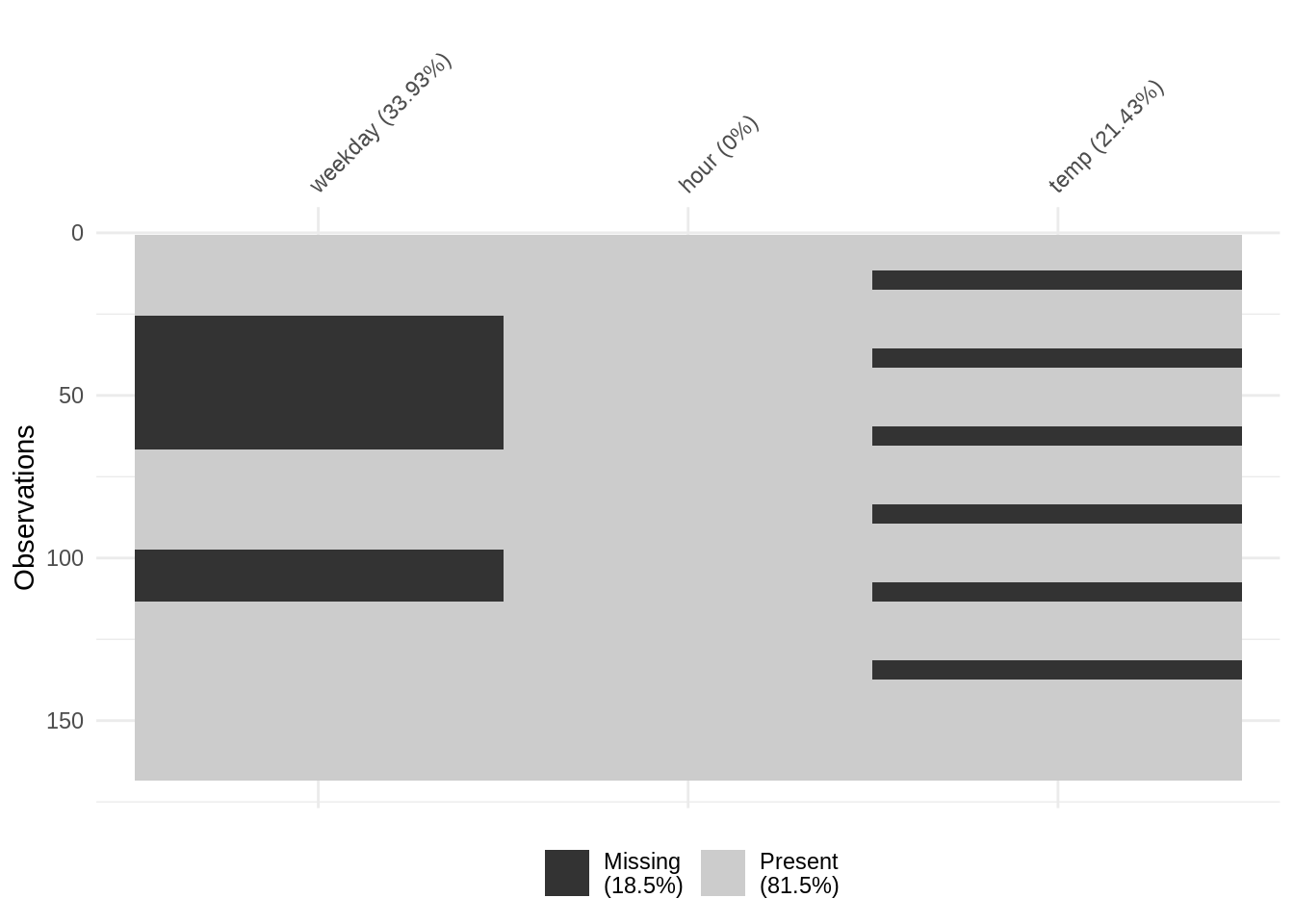
Below are the functions we will use in this section to explore missingness in spans and streaks
gg_miss_span(): visualise the proportion of missing values by spanmiss_var_span(): table containing counts and proportions of missingness by spanmiss_var_run(): table containing lengths of streaks for missing and non-missing values in the data
5.0.1 Missingness in spans
The gg_miss_span() and miss_var_span() functions in naniar provide visual and tabular summaries of missing values in user-specified spans, or equally-sized periods, within the data.
Let’s show the data we visualised using vis_miss() in figure @ref(fig:plot-span-streak):
knitr::kable(head(dat_span, 26))| weekday | hour | temp |
|---|---|---|
| 1 | 1 | 22 |
| 1 | 2 | 18 |
| 1 | 3 | 27 |
| 1 | 4 | 27 |
| 1 | 5 | 25 |
| 1 | 6 | 27 |
| 1 | 7 | 21 |
| 1 | 8 | 22 |
| 1 | 9 | 21 |
| 1 | 10 | 19 |
| 1 | 11 | 27 |
| 1 | 12 | NA |
| 1 | 13 | NA |
| 1 | 14 | NA |
| 1 | 15 | NA |
| 1 | 16 | NA |
| 1 | 17 | NA |
| 1 | 18 | 16 |
| 1 | 19 | 14 |
| 1 | 20 | 20 |
| 1 | 21 | 14 |
| 1 | 22 | 11 |
| 1 | 23 | 25 |
| 1 | 24 | 19 |
| 2 | 1 | 20 |
| NA | 2 | 12 |
This is a fake dataset that contains information of weekday (1 through to 7), the hour of the day, and the temperature recorded that day.
We noticed before the regular “stripey” patterns of missingness in Figure @ref(fig:plot-span-streak) in the temp variable. Although we have information on the amount of missingness in this variable from vis_miss, we do not have further information on how often it occurs. Let’s learn more about this by using the gg_miss_span() function:
gg_miss_span(data = dat_span,
             var = temp,
             span_every = 12)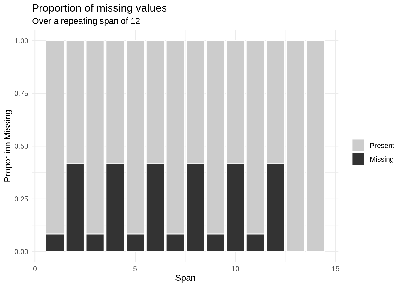
What is figure @ref(fig:gg-miss-span-dat)) showing us? We have calculated the missingness in the temp variable, where the missingness is calculated over some repeating span. The span_every argument of 12 means missing frequency and proportion will be evaluated every 12 row. So, for observations 1 to 12, then 13-24, then 25-36, and so on. Each of the spans is indicated on the x-axis; and on the y-axis, we see the proportion of values within each span.
How do we interpret figure @ref(fig:gg-miss-span-dat)? In this case, since the data occurs every hour, with a span of 12, we are looking at the proportion of missingness at every 12 hour interval. Notice we get a strong repeating pattern of missingness, but it seems a bit lopsided, like the proportion of missingness is bleeding over from hours 12-15, perhaps? What happens if we explore every 24 hours?
gg_miss_span(data = dat_span,
             var = temp,
             span_every = 24)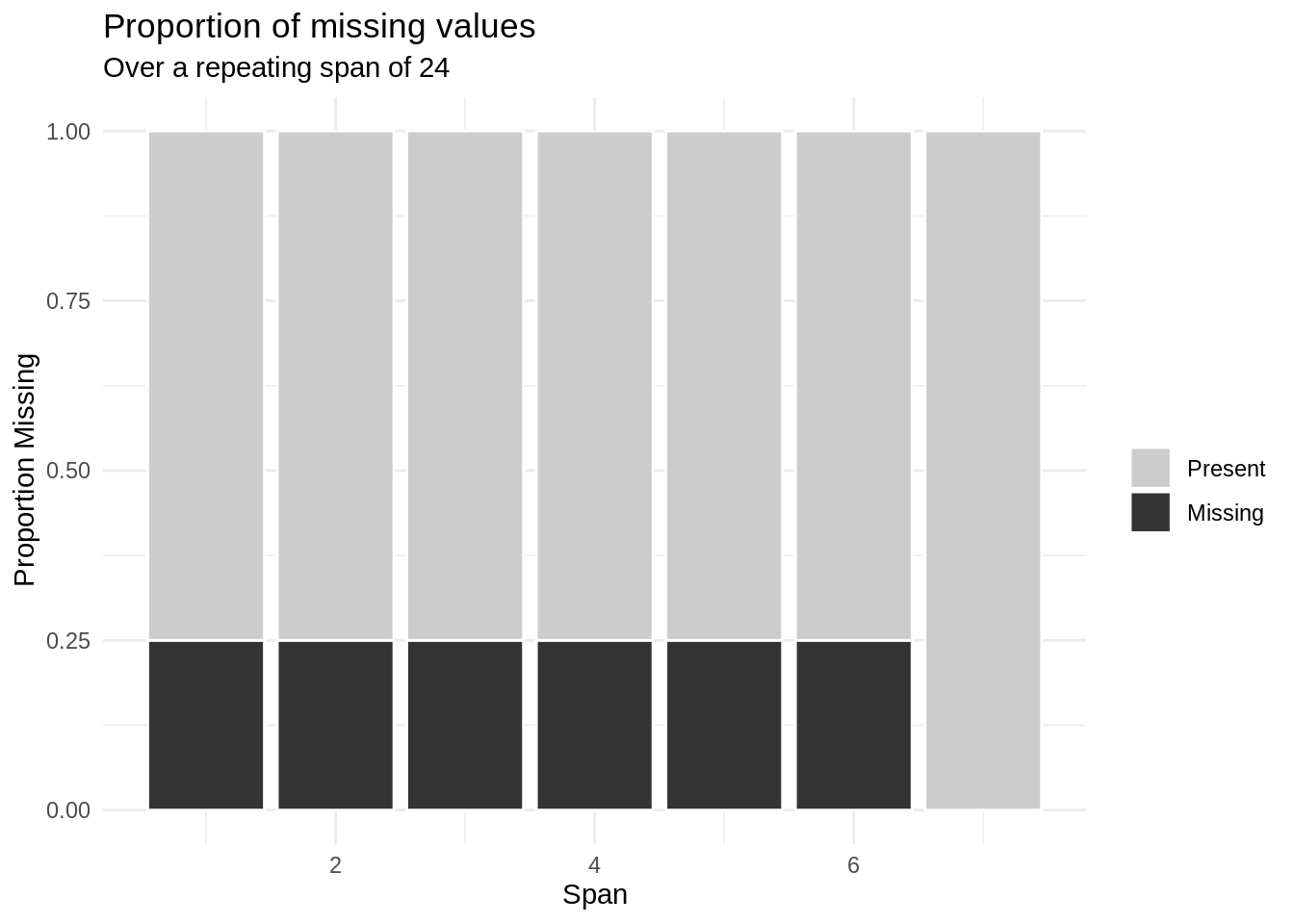
Ah! Notice that we’re getting some missingness every 12 hours.
5.0.2 Example: Pedestrian data
Let’s consider the pedestrian dataset in naniar, which contains “hourly counts of pedestrians from 4 sensors around Melbourne”. See the dataset documentation (?pedestrian) for further details and citation.
glimpse(pedestrian)Rows: 37,700
Columns: 9
$ hourly_counts <int> 883, 597, 294, 183, 118, 68, 47, 52, 120, 333, 761, 1352…
$ date_time <dttm> 2016-01-01 00:00:00, 2016-01-01 01:00:00, 2016-01-01 02…
$ year <int> 2016, 2016, 2016, 2016, 2016, 2016, 2016, 2016, 2016, 20…
$ month <ord> January, January, January, January, January, January, Ja…
$ month_day <int> 1, 1, 1, 1, 1, 1, 1, 1, 1, 1, 1, 1, 1, 1, 1, 1, 1, 1, 1,…
$ week_day <ord> Friday, Friday, Friday, Friday, Friday, Friday, Friday, …
$ hour <int> 0, 1, 2, 3, 4, 5, 6, 7, 8, 9, 10, 11, 12, 13, 14, 15, 16…
$ sensor_id <int> 2, 2, 2, 2, 2, 2, 2, 2, 2, 2, 2, 2, 2, 2, 2, 2, 2, 2, 2,…
$ sensor_name <chr> "Bourke Street Mall (South)", "Bourke Street Mall (South…An aside on choosing interval size
Importantly, observations in the
pedestriandata are recorded at equal hourly intervals, making equal spans of interest. If data are recorded at non-equal intervals, or intermittently, investigating missingness by span may not be meaningful or informative. This is because when we explore something by a fixed interval, we want the data to have meaning at that fixed interval. If we explored our data that occurs at hourly intervals in 10 hour intervals, it might be hard to understand why 10 hours is chosen, as it might not make sense as it goes on from hour 0-10, 11-20, 21-30, and so on. Whereas if instead 12 hour or 24 hour intervals were chosen then those naturally break down into the first and second half of a day. So, all this is to say that it is important to think carefully on interval size when investigating equally-sized spans data.
Since the pedestrian observations are recording at equal intervals (and therefore spans are meaningful), it may be useful to explore the prevalence of missing values within repeated, equally-sized spans.
In the example below, missingness in the hourly_counts variable from pedestrian is calculated over repeating spans; the span_every argument indicates that missingness should be evaluated for each span of 672 observations. Why 672? Well there aer 168 hours every 7 days, and 672 hours every 4 weeks - so this shows us the amount of missing data every 4 weeks.
gg_miss_span(pedestrian, hourly_counts, span_every = 672)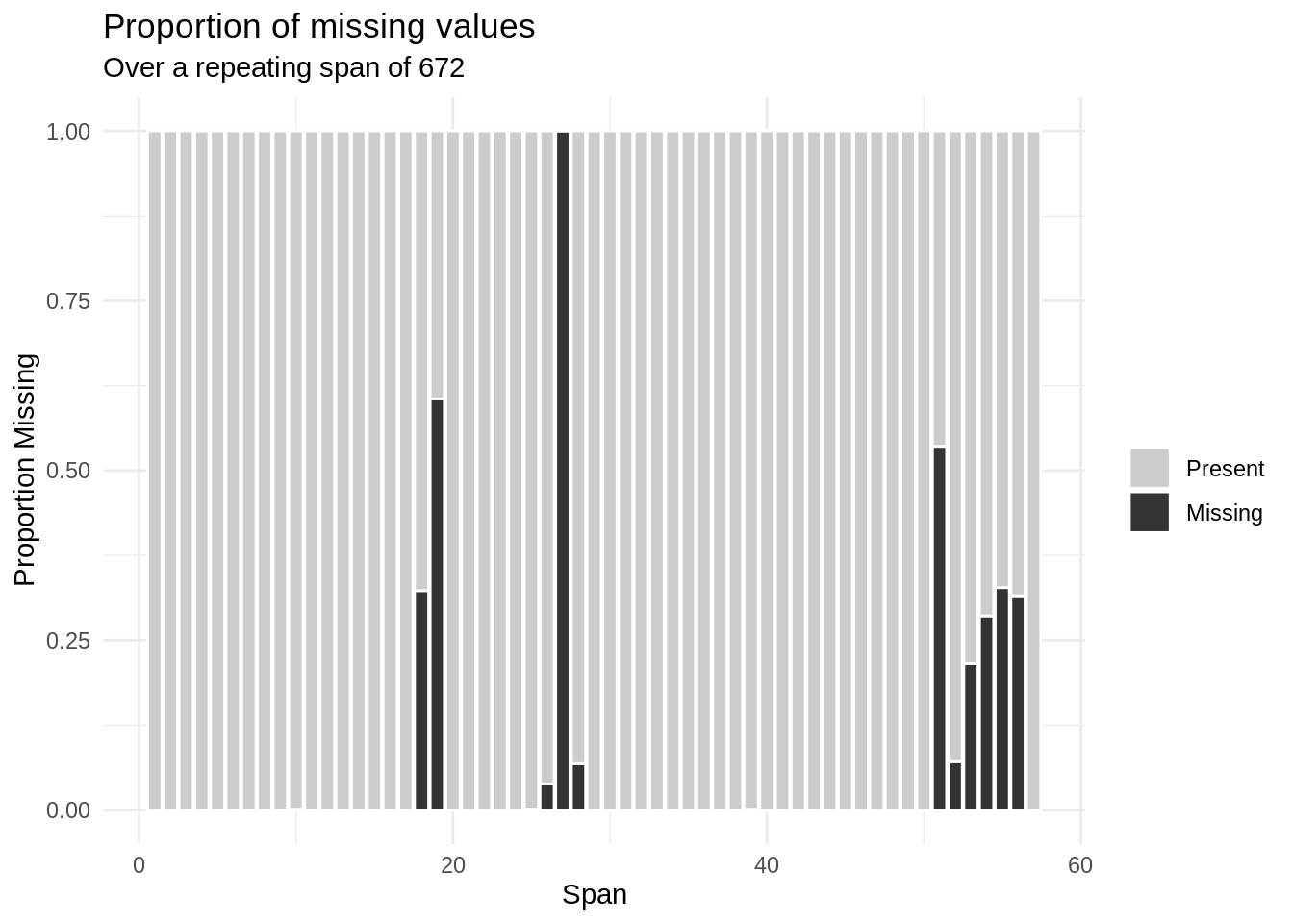
How do we interpret the output above from gg_miss_span? We see that with a selected span size of 672, there are a total of 56 spans included, since there are 37,700 rows (672 * 56 = 37,632). Each of the spans is indicated on the x-axis; on the y-axis, the proportion of values within each span is indicated.
We can get the tabular format of the data put into gg_miss_span with miss_var_span:
miss_var_span(pedestrian,
              var = hourly_counts,
              span_every = 672)
# A tibble: 57 × 6
span_counter n_miss n_complete prop_miss prop_complete n_in_span
<int> <int> <int> <dbl> <dbl> <int>
1 1 0 672 0 1 672
2 2 0 672 0 1 672
3 3 0 672 0 1 672
4 4 0 672 0 1 672
5 5 0 672 0 1 672
6 6 0 672 0 1 672
7 7 0 672 0 1 672
8 8 0 672 0 1 672
9 9 0 672 0 1 672
10 10 1 671 0.00149 0.999 672
# … with 47 more rowsNotice that the outputs for the two examples above reveal the same information, either in visual or tabular form. Let’s interpret some values to see how they align:
- The first column in the graph from
gg_miss_spanabove does not appear to contain any missing values; that is confirmed in the first row frommiss_var_spanabove showing that inspan_counter1 there are 0 missing values - The tenth column in the
gg_miss_spangraph (span_counter10) has some proportion of missing values within the span; from themiss_var_spanoutput we can see that there is 1 missing values in that span (0.1% missing)
5.0.2.1 Missingness within spans, by group
You can further break down missingness within spans by group, by faceting with gg_miss_span or grouping data prior to using miss_var_span.
For example, the above investigation of missingness for hourly_counts in pedestrian, using a span size of 168 cases (1 week), can be faceted by sensor_name as follows:
gg_miss_span(data = pedestrian,
             var = hourly_counts,
             span_every = 168,
             facet = sensor_name)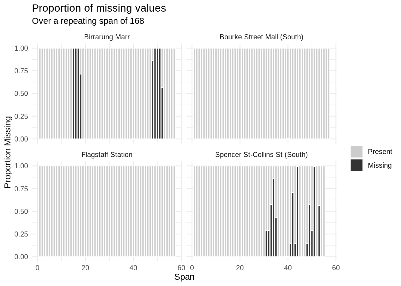
We can produce the analogous tabular version of that result by grouping data (group_by(month)) before miss_var_summary as follows:
pedestrian %>%
  group_by(sensor_name) %>%
  miss_var_span(var = hourly_counts,
                span_every = 168)
# A tibble: 226 × 7
# Groups: sensor_name [4]
sensor_name span_counter n_miss n_complete prop_miss prop_complete n_in_span
<chr> <int> <int> <int> <dbl> <dbl> <int>
1 Bourke Stre… 1 0 168 0 1 168
2 Bourke Stre… 2 0 168 0 1 168
3 Bourke Stre… 3 0 168 0 1 168
4 Bourke Stre… 4 0 168 0 1 168
5 Bourke Stre… 5 0 168 0 1 168
6 Bourke Stre… 6 0 168 0 1 168
7 Bourke Stre… 7 0 168 0 1 168
8 Bourke Stre… 8 0 168 0 1 168
9 Bourke Stre… 9 0 168 0 1 168
10 Bourke Stre… 10 0 168 0 1 168
# … with 216 more rowsHow do we interpret these outputs grouped by sensor_name? Well, this is very interesting - it looks like there is only missingness in two of the sensors, Birrarung Marr and Spencer St - Collins St (South). Within those two, it looks like some of the sensors were down a few weeks. Let’s filter down to “Birrarun Marr” and explore that further, facetting by month and showing the weekly amounts of missinginess:
pedestrian %>%
  filter(sensor_name == "Birrarung Marr") %>%
  gg_miss_span(var = hourly_counts,
               span_every = 168,
               facet = month)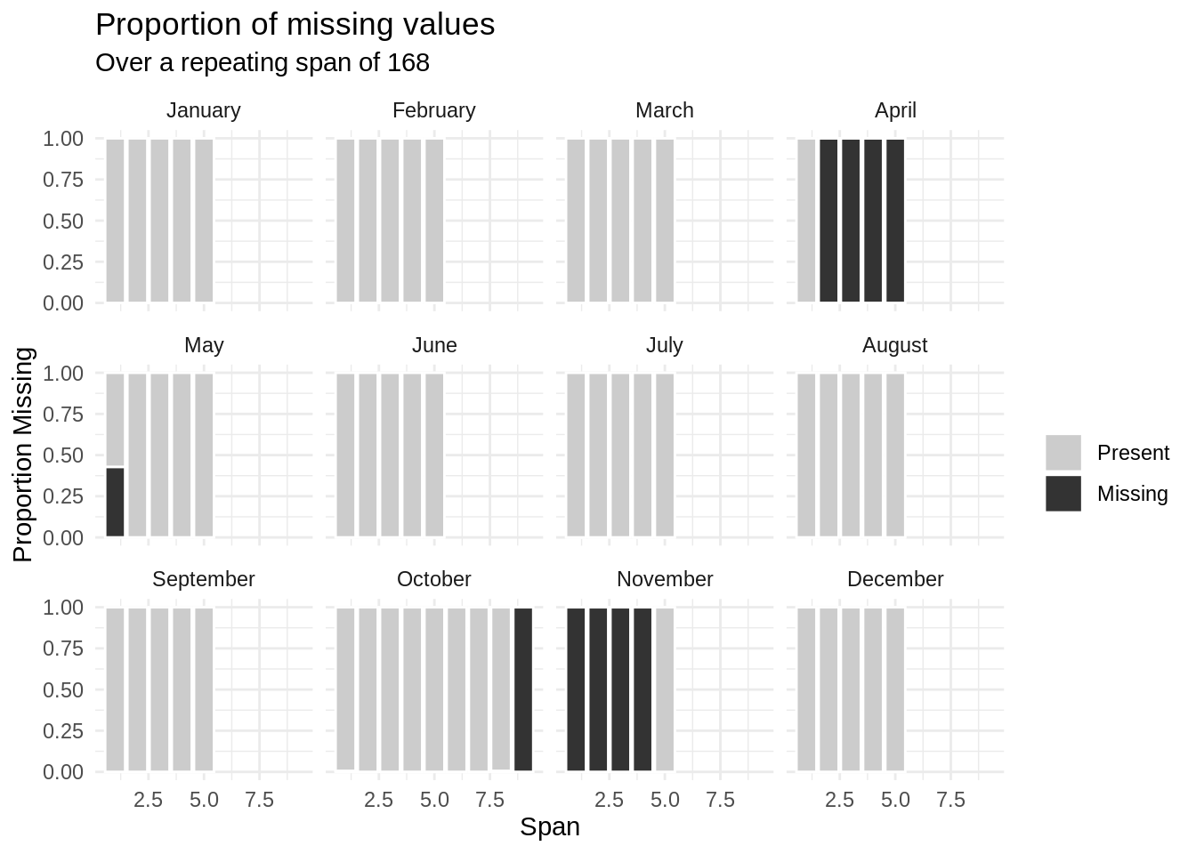
It looks like there was an outage from the second week in April until the first week of May, then into October and November.
Aside: What happens to span remainders
What happens if you have a span that doens’t fit into the number of rows of a dataset? For example, if you have spans of 50, and there are 168 rows? The final span, which would be have rows 151-168, and the proportion of missingness will be calculated as that set of data.
5.0.3 Streaks of missingness
Another way to explore patterns in missingness is by lengths of streaks for non-missing and missing values. For any vector (or variable in a data frame), the miss_var_run function in naniar returns the length of runs for complete and missing values. This can be particularly useful for finding repeating patterns of missingness.
For example, to explore streaks of missingness in the hourly_counts variable from the pedestrians data we can use:
miss_var_run(pedestrian, hourly_counts)# A tibble: 35 × 2
run_length is_na
<int> <chr>
1 6628 complete
2 1 missing
3 5250 complete
4 624 missing
5 3652 complete
6 1 missing
7 1290 complete
8 744 missing
9 7420 complete
10 1 missing
# … with 25 more rowsWhat can we learn from the output above? There is a long initial streak (n = 6,628) of complete values for hourly_counts, the a single missing value, followed by another long streak of complete values (n = 5,250) before a more substantial streak of missingness (n = 624), and so on.
We can use miss_var_run with group_by to explore runs of missing data within months:
pedestrian %>%
  group_by(month) %>%
  miss_var_run(var = hourly_counts)
# A tibble: 51 × 3
# Groups: month [12]
month run_length is_na
<ord> <int> <chr>
1 January 2976 complete
2 February 2784 complete
3 March 2976 complete
4 April 888 complete
5 April 552 missing
6 April 1440 complete
7 May 744 complete
8 May 72 missing
9 May 2160 complete
10 June 2880 complete
# … with 41 more rowsOr within sensors:
pedestrian %>%
  group_by(sensor_name) %>%
  miss_var_run(var = hourly_counts)
# A tibble: 38 × 3
# Groups: sensor_name [4]
sensor_name run_length is_na
<chr> <int> <chr>
1 Bourke Street Mall (South) 6628 complete
2 Bourke Street Mall (South) 1 missing
3 Bourke Street Mall (South) 2898 complete
4 Birrarung Marr 2352 complete
5 Birrarung Marr 624 missing
6 Birrarung Marr 3652 complete
7 Birrarung Marr 1 missing
8 Birrarung Marr 1290 complete
9 Birrarung Marr 744 missing
10 Birrarung Marr 792 complete
# … with 28 more rowsor within each month for each sensor name:
pedestrian %>%
  group_by(month,
           sensor_name) %>%
  miss_var_run(var = hourly_counts)
# A tibble: 82 × 4
# Groups: month, sensor_name [48]
month sensor_name run_length is_na
<ord> <chr> <int> <chr>
1 January Bourke Street Mall (South) 744 complete
2 February Bourke Street Mall (South) 696 complete
3 March Bourke Street Mall (South) 744 complete
4 April Bourke Street Mall (South) 720 complete
5 May Bourke Street Mall (South) 744 complete
6 June Bourke Street Mall (South) 720 complete
7 July Bourke Street Mall (South) 744 complete
8 August Bourke Street Mall (South) 744 complete
9 September Bourke Street Mall (South) 720 complete
10 October Bourke Street Mall (South) 52 complete
# … with 72 more rowsWe can imagine questions that might arise when considering streaks of missingness: Were there changes in sampling protocols? Did the person, equipment, or study site change? Did funding get cut? Any of these might help to understand why values are missing, an important question when working with incomplete data and useful when deciding how to deal with missing values in analyses.