4 Missingness by variables (columns) and cases (rows)

This book contains both practical guides on exploring missing data, as well as some of the deeper details of how naniar works to help you better explore your missing data. A large component of this book are the exercises that accompany each section in each chapter.

library(naniar)
library(dplyr)

Once we have a broad overview of missingness in the data, the next step is to explore how missingness exists at finer resolution within variables and cases. You might also refer to variables and cases as “columns” and “rows”, but for consistency, we will use “variables” and “cases”. Below are the functions we will use in this section to explore missingness in variables and cases:

Functions to explore missingness by variable:

gg_miss_var: visualise frequency of missingness by variable
miss_var_summary: table of missingness frequency by variable
miss_var_table: table of missing frequencies by variable

Functions to explore missingness by case:

gg_miss_case: visualise frequency of missing values by case
miss_case_summary: table of missingness frequency by case
miss_case_table: table of missing frequencies by case

An aside

You might notice that there is a lot of similarity in the naming and purpose of each of these functions - this is intentional! They are designed to have names that help cue your understanding or purpose of the next task. There are many other functions that start with miss_var_ and miss_case, and gg_miss. These functions have been written like so to facilitate exploration of new functions, and also to reduce the cognitive burden of trying to remember what a function is called. Instead, you can focus on, “I want to explore missings by variable - I’ll start by exploring what is in miss_var”, and if you want to create visualisations, you can use gg_miss_* to explore available options.

4.0.1 Missingness within variables

The gg_miss_var and miss_var_summary functions in naniar return visual and tabular summaries, respectively, of missingness within each variable. For example, gg_miss_var applied to the airquality returns a lollipop plot with the frequency of missingness on the x axis, and the variable name on the y-axis:

gg_miss_var(airquality)

Warning: It is deprecated to specify `guide = FALSE` to remove a guide. Please
use `guide = "none"` instead.

Note that the visualisation is ordered (high-to-low) by variable highest frequency of missing values.

To instead create a table with the number and percentage of missing values for each variable (column), use miss_var_summary:

miss_var_summary(airquality)

# A tibble: 6 × 3
  variable n_miss pct_miss
  <chr>     <int>    <dbl>
1 Ozone        37    24.2 
2 Solar.R       7     4.58
3 Wind          0     0   
4 Temp          0     0   
5 Month         0     0   
6 Day           0     0

We see that miss_var_summary() returns a data frame where each row in the output contains the total number (n_miss) and percentage (pct_miss) of missing values for each variable in the original data. Note that miss_var_summary and gg_miss_summary give us the same information, presented differently: the values in the miss_var_summary table for each variable align with the frequency of missingness indicated on the x-axis from the gg_miss_var output.

An example of how to interpret missingness within variables from miss_var_summary and gg_miss_var is:

An overview of missingness in the in the airquality dataset (n_obs = 153). The Ozone variable has the highest frequency of missing values (n_missing = 37; percent missing = 24.2%), followed by Solar.R (n_missing = 7; percent missing = 4.6%). The remaining four variables (Wind, Temp, Month, and Day) contain no missing values.

4.0.1.1 Missingness by variable, within groups

We can explore missingness in detail within each variable by using the facet argument, which will split each plot into one facet per level of a variable. The example below shows the number of missing values in each variable (gg_miss_var) in the airquality data, now broken up by the different levels in Month.

gg_miss_var(airquality, facet = Month)

Warning: It is deprecated to specify `guide = FALSE` to remove a guide. Please
use `guide = "none"` instead.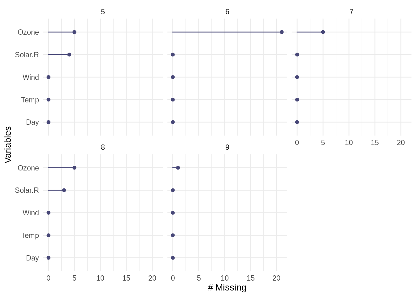

In the graph above, we can see there is now a separate panel for each month appearing in the data (5, 6, 7, 8, and 9), to allow for a comparison of missingness by variable across and within each month.

The same information can be reported in tabular form by miss_var_summary in combination with group_by to designate which variable to group by. For example, we parse missingness by Month in the airquality dataset:

airquality %>%
  group_by(Month) %>%
  miss_var_summary()

# A tibble: 25 × 4
# Groups:   Month [5]
   Month variable n_miss pct_miss
   <int> <chr>     <int>    <dbl>
 1     5 Ozone         5     16.1
 2     5 Solar.R       4     12.9
 3     5 Wind          0      0  
 4     5 Temp          0      0  
 5     5 Day           0      0  
 6     6 Ozone        21     70  
 7     6 Solar.R       0      0  
 8     6 Wind          0      0  
 9     6 Temp          0      0  
10     6 Day           0      0  
# … with 15 more rows

Here, we see the Ozone variable contains 5 missing values for Month 5, and 21 missing values for Month 6.

4.0.1.2 `miss_var_table`

It can be useful to explore how often (i.e., for how many variables or cases) different frequencies of missingness occur. That’s kind of a brainful, so here are some example questions we might ask:

“How many variables contain zero missing values?”

“How many variables contain one missing values?”

“How many variables contain two missing values?”

The miss_var_table() function tells us how many variables contain different frequencies of missingness. For example, we can use miss_var_table with our airquality data to calculate and return the number of variables with different frequencies of missing values:

miss_var_table(airquality)

# A tibble: 3 × 3
  n_miss_in_var n_vars pct_vars
          <int>  <int>    <dbl>
1             0      4     66.7
2             7      1     16.7
3            37      1     16.7

The table returned above tells us the following:

Row 1 in output table: four variables (n_vars = 4, or 66.7% of all variables) contain zero missing values (n_miss_in_var = 0)
Row 2 in output table: one variable (n_vars = 1, or 16.7% of all variables) contains 7 missing values (n_miss_in_var = 7)
Row 3 in output table: one variable (n_vars = 1, or 16.7% of all variables) contains 37 missing values (n_miss_in_var = 37)

Writing this as a brief summary, we might write:

Four variables (~ 66.7% of columns) contain no missing values; one variable contains 7 missing values, and one variable contains 37 missing values.

4.0.2 Missingness by case (rows)

The gg_miss_case() and miss_case_summary() functions return visual and tabular summaries of missingness by case (row) within the data. For example, to visualize missingness by case:

gg_miss_case(airquality)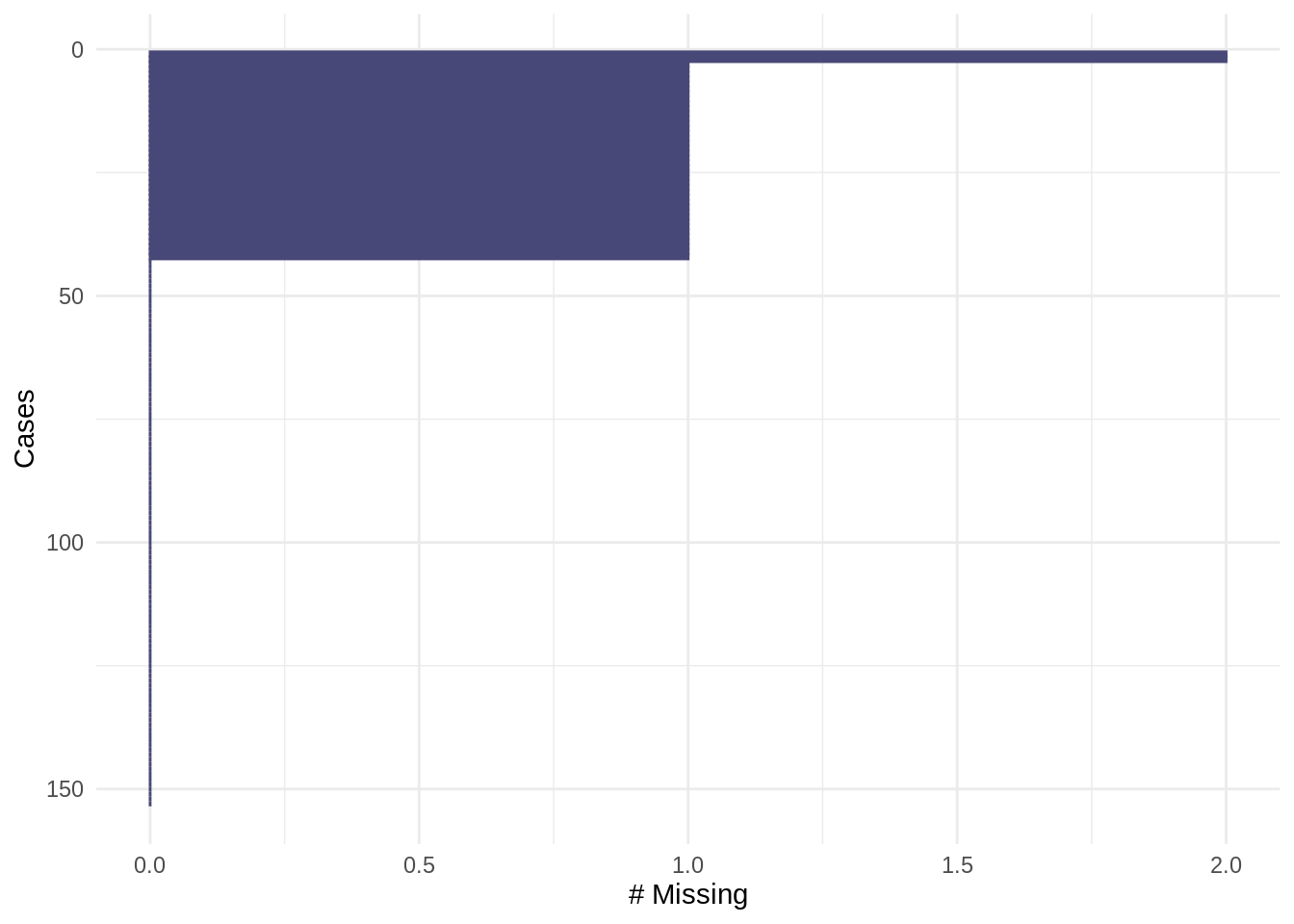

Note that the visualisation is similarly ordered (high-to-low) by case(s) with the highest frequency of missing values. The ordering in gg_miss_case can be turned off with option, order_cases = FALSE, which will keep the order of the data as presented to the function.

gg_miss_case(airquality, order_cases = FALSE)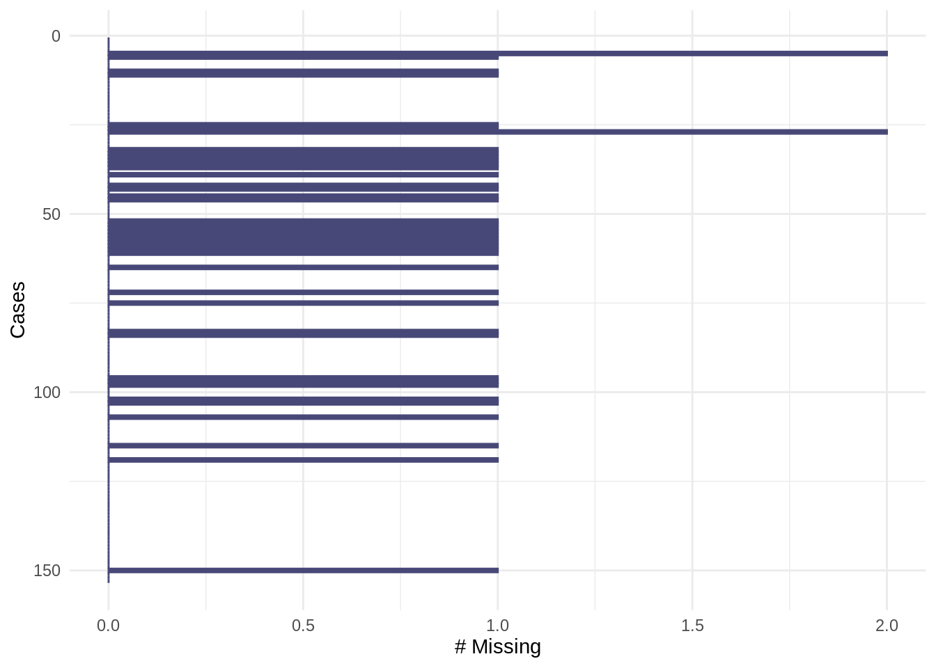

For a tabular summary of missingness by case, use miss_case_summary. The miss_case_summary function returns a summary data frame with the frequency and percentage of missing values for each case (row) in the original data, arranged by decreasing missingness.

miss_case_summary(airquality)

# A tibble: 153 × 3
    case n_miss pct_miss
   <int>  <int>    <dbl>
 1     5      2     33.3
 2    27      2     33.3
 3     6      1     16.7
 4    10      1     16.7
 5    11      1     16.7
 6    25      1     16.7
 7    26      1     16.7
 8    32      1     16.7
 9    33      1     16.7
10    34      1     16.7
# … with 143 more rows

In the example output above, the case column contains the original row number (case) in the data, and the frequency and percent missing is returned for each case. Here, we can interpret the first two rows of this summary as follows:

In the airquality dataset, cases 5 and 27 - the 5^th and 27^th rows in the original dataset - each contain 2 missing values (i.e. 2 of 6 values, or 33.3%, in each row are missing).

4.0.2.1 Missingness by case, within groups

Missingness by case can be further explored within groups by faceting (with gg_miss_case) or in combination with group_by.

To visualize missingness by case within groups, add a faceting variable to the argument facet. The example below shows the number of missing values in each case (gg_miss_case) in the airquality data, faceted by Month.

gg_miss_case(airquality, facet = Month)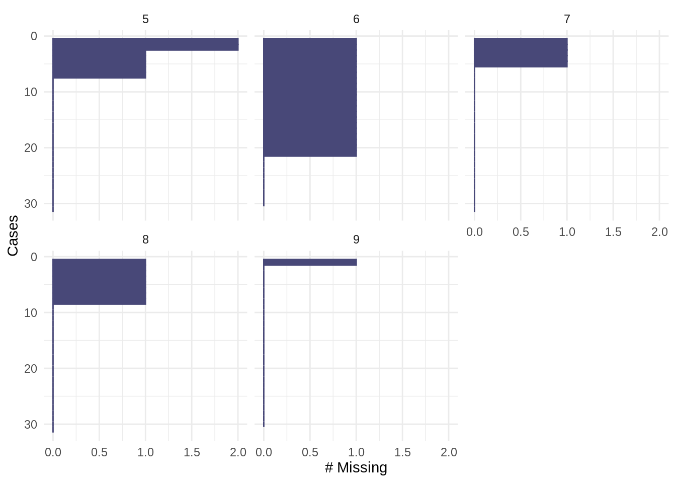

To return the above data (missingness by case, separated by each level in Month) in tabular form, use miss_case_summary in combination with group_by:

airquality %>%
  group_by(Month) %>%
  miss_case_summary()

# A tibble: 153 × 4
# Groups:   Month [5]
   Month  case n_miss pct_miss
   <int> <int>  <int>    <dbl>
 1     5     5      2       40
 2     5    27      2       40
 3     5     6      1       20
 4     5    10      1       20
 5     5    11      1       20
 6     5    25      1       20
 7     5    26      1       20
 8     5     1      0        0
 9     5     2      0        0
10     5     3      0        0
# … with 143 more rows

4.0.2.2 `miss_case_table`

We may want to know:

“How many cases are complete (no missing values)?”

“How many cases have one missing value?”

“How many cases have two missing values?”

The miss_case_table function in naniar tells us how many cases contain different frequencies of missingness. The example below returns the number of cases (rows) in the airquality data that contain different numbers of missing values:

miss_case_table(airquality)

# A tibble: 3 × 3
  n_miss_in_case n_cases pct_cases
           <int>   <int>     <dbl>
1              0     111     72.5 
2              1      40     26.1 
3              2       2      1.31

We could summarize the output above as follows:

The majority of cases (72.5%) are complete, 26.1% of cases contain one missing value, and ~1.3% of cases contain two missing values; no cases contain more than two missing values.

Using the naniar functions in this section, we got a more detailed view of missingness within variables and cases. In the next section, we investigate patterns of missingness streaks and spans.