14 Imputing with different models

This book contains both practical guides on exploring missing data, as well as some of the deeper details of how naniar works to help you better explore your missing data. A large component of this book are the exercises that accompany each section in each chapter.

There are many imputation packages in R. We are going to focus on using the simputation package by Mark van der Loo. simputation provides a simple interface to many imputation models. We will impute values using a linear model, using the function impute_lm().

Building a good imputation model is super important, but it is a complex topic - there is as much to building a good imputation model as there is for building a good statistical model. We focus on how to build up different imputation models and assess and compare them.

library(naniar)
library(tidyverse)

── Attaching packages ─────────────────────────────────────── tidyverse 1.3.1 ──

✔ ggplot2 3.3.6     ✔ purrr   0.3.4
✔ tibble  3.1.7     ✔ dplyr   1.0.9
✔ tidyr   1.2.0     ✔ stringr 1.4.0
✔ readr   2.1.2     ✔ forcats 0.5.1

── Conflicts ────────────────────────────────────────── tidyverse_conflicts() ──
✖ dplyr::filter() masks stats::filter()
✖ dplyr::lag()    masks stats::lag()

library(simputation)


Attaching package: 'simputation'

The following object is masked from 'package:naniar':

    impute_median

When you develop imputation models, it is a good idea to try out a few different models, to see how the imputed values change according to your assumptions. In this chapter, we are going to impute data using linear regression.

An Aside: Running many models used to make me feel like I was cheating

I (Nick), studied psychology in my undergraduate degree. The training for statistics was very focussed on developing a theory first, then designing a study design and appropriate statistial model. You’d then collect data, and turn the cranks on the statistical (usually ANOVA) machinery and out would come your answer - is the result significant: yes, or no? When I started my PhD in statistics, the idea of exploring many different fits to your data felt strange, and like I was cheating! Fitting many models in psych would have felt like we were chasing significance, and that I’d be labelled a “p-value hacker”. In these cases, however, we weren’t conducting controlled experiments to test a theory, rather we were exploring data that wasn’t collected with a research question in mind. In our case with missing data, fitting many models is about trying to identify the most sensible values that could have existed, so that we can draw sensible inferences on the data.

14.1 How imputation using a linear model works

We previously explored using mean imputation. This is generally a bad imputation method to use, as it artificially increases the mean and reduces variance, so you aren’t capturing the natural variation in the data. Similar to how the mean was imputed, we can use a linear model to impute data. This can take into account some features of the data, to better predict missing values.

To impute values using a linear model, we use impute_lm from simputation. Let’s create some fake data, df:

df <- tibble(
  y = c(2.67, 3.87, NA, 5.21, NA),
  x1 = c(2.43, 3.55, 2.9, 2.72, 4.29),
  x2 = c(3.27, 1.45, 1.49, 1.84, 1.15)
  )

df

# A tibble: 5 × 3
      y    x1    x2
  <dbl> <dbl> <dbl>
1  2.67  2.43  3.27
2  3.87  3.55  1.45
3 NA     2.9   1.49
4  5.21  2.72  1.84
5 NA     4.29  1.15

Now to use impute_lm(), we specify the variable we would like to impute on as the y or dependent variable, just as you would with a linear model. On the right hand side of the formula are the variables we would like to use to inform the imputations on the right hand side. This returns a data frame with imputed values in y:

df %>% 
  impute_lm(y ~ x1 + x2)

# A tibble: 5 × 3
      y    x1    x2
* <dbl> <dbl> <dbl>
1  2.67  2.43  3.27
2  3.87  3.55  1.45
3  5.54  2.9   1.49
4  5.21  2.72  1.84
5  2.56  4.29  1.15

Of course, we need to use nabular to make sure we can track what values were imputed in y_NA:

df %>% 
  nabular() %>%
  impute_lm(y ~ x1 + x2)

# A tibble: 5 × 6
      y    x1    x2 y_NA  x1_NA x2_NA
* <dbl> <dbl> <dbl> <fct> <fct> <fct>
1  2.67  2.43  3.27 !NA   !NA   !NA  
2  3.87  3.55  1.45 !NA   !NA   !NA  
3  5.54  2.9   1.49 NA    !NA   !NA  
4  5.21  2.72  1.84 !NA   !NA   !NA  
5  2.56  4.29  1.15 NA    !NA   !NA

14.2 Using `impute_lm`

Using airquality data, we can impute the values in Solar.R using Wind, Temp, and Month, and chain another imputation step in to impute Ozone with the same variables. This gives us imputations like the following:

aq_imp_lm <- airquality %>%
  nabular() %>%
  add_label_shadow() %>%
  as.data.frame() %>%
  impute_lm(Solar.R ~ Wind + Temp + Month) %>%
  impute_lm(Ozone ~ Wind + Temp + Month) %>% 
  as_tibble()

aq_imp_lm

# A tibble: 153 × 13
   Ozone Solar.R  Wind  Temp Month   Day Ozone_NA Solar.R_NA Wind_NA Temp_NA
   <dbl>   <dbl> <dbl> <int> <int> <int> <fct>    <fct>      <fct>   <fct>  
 1 41       190    7.4    67     5     1 !NA      !NA        !NA     !NA    
 2 36       118    8      72     5     2 !NA      !NA        !NA     !NA    
 3 12       149   12.6    74     5     3 !NA      !NA        !NA     !NA    
 4 18       313   11.5    62     5     4 !NA      !NA        !NA     !NA    
 5 -9.04    138.  14.3    56     5     5 NA       NA         !NA     !NA    
 6 28       178.  14.9    66     5     6 !NA      NA         !NA     !NA    
 7 23       299    8.6    65     5     7 !NA      !NA        !NA     !NA    
 8 19        99   13.8    59     5     8 !NA      !NA        !NA     !NA    
 9  8        19   20.1    61     5     9 !NA      !NA        !NA     !NA    
10 35.2     194    8.6    69     5    10 NA       !NA        !NA     !NA    
# … with 143 more rows, and 3 more variables: Month_NA <fct>, Day_NA <fct>,
#   any_missing <chr>

Note: the as.data.frame() is necessary for the time being due to a workaround with simputation. Nick is hoping to arrive on a better solution to this soon.

14.2.1 Tracking missing values

An important part of imputing data is using the nabular() and add_label_shadow() functions. Without them, we can’t identify which values were missing! So, let’s recap what they do.

nabular() adds the variables with _NA to the data

[TODO: image of this]

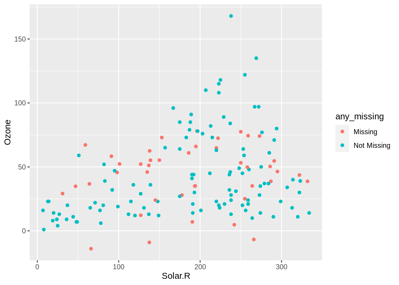
add_label_shadow() adds a variable, any_missing, with values “Missing” or “Not Missing”.We can use ggplot to show the imputed values, by setting colour = any_missing in a ggplot.

aq_imp_lm <- airquality %>%
  nabular() %>%
  add_label_missings() %>%
  as.data.frame() %>% 
  impute_lm(Solar.R ~ Wind + Temp + Month) %>%
  impute_lm(Ozone ~ Wind + Temp + Month) %>% 
  as_tibble()

aq_imp_lm

# A tibble: 153 × 13
   Ozone Solar.R  Wind  Temp Month   Day Ozone_NA Solar.R_NA Wind_NA Temp_NA
   <dbl>   <dbl> <dbl> <int> <int> <int> <fct>    <fct>      <fct>   <fct>  
 1 41       190    7.4    67     5     1 !NA      !NA        !NA     !NA    
 2 36       118    8      72     5     2 !NA      !NA        !NA     !NA    
 3 12       149   12.6    74     5     3 !NA      !NA        !NA     !NA    
 4 18       313   11.5    62     5     4 !NA      !NA        !NA     !NA    
 5 -9.04    138.  14.3    56     5     5 NA       NA         !NA     !NA    
 6 28       178.  14.9    66     5     6 !NA      NA         !NA     !NA    
 7 23       299    8.6    65     5     7 !NA      !NA        !NA     !NA    
 8 19        99   13.8    59     5     8 !NA      !NA        !NA     !NA    
 9  8        19   20.1    61     5     9 !NA      !NA        !NA     !NA    
10 35.2     194    8.6    69     5    10 NA       !NA        !NA     !NA    
# … with 143 more rows, and 3 more variables: Month_NA <fct>, Day_NA <fct>,
#   any_missing <chr>

ggplot(aq_imp_lm,
       aes(x = Solar.R,
           y = Ozone,
           colour = any_missing)) +
  geom_point()

Without the any_missing variable, we could only identify the missings of one variable: Solar.R_NA or Ozone_NA.

14.3 Evaluating imputations: Evaluating and comparing imputations

aq_imp_small <- airquality %>%
  nabular() %>%
  as.data.frame() %>% 
  impute_lm(Ozone ~ Wind + Temp) %>%
  impute_lm(Solar.R ~ Wind + Temp) %>%
  add_label_shadow()
  
aq_imp_large <- airquality %>%
  nabular() %>%
  as.data.frame() %>% 
  impute_lm(Ozone ~ Wind + Temp + Month + Day) %>%
  impute_lm(Solar.R ~ Wind + Temp + Month + Day)  %>%
  add_label_shadow()

When you build up an imputation model, it is good practice to compare it to an alternative method. Let’s compare two linear regression imputation models. The first with two variables: Wind, and Temperature, and the second with four: Wind, Temperature, Month, and Day.

To facilitate comparing models, we put them into the same dataframe, by binding their rows together using bind_rows from dplyr package.

bound_models <- bind_rows(
  small = aq_imp_small,
  large = aq_imp_large,
  .id = "imp_model"
  ) %>% 
  as_tibble()

To help us identify which data came from which imputation process, we use the .id argument to add a new column that identifies them. By writing small = aq_imp_small and large = aq_imp_large, we can then use .id = "imp_model". This creates a dataset of all the imputations with an extra column, imp_model.

head(bound_models)

# A tibble: 6 × 14
  imp_model Ozone Solar.R  Wind  Temp Month   Day Ozone_NA Solar.R_NA Wind_NA
  <chr>     <dbl>   <dbl> <dbl> <int> <int> <int> <fct>    <fct>      <fct>  
1 small      41      190    7.4    67     5     1 !NA      !NA        !NA    
2 small      36      118    8      72     5     2 !NA      !NA        !NA    
3 small      12      149   12.6    74     5     3 !NA      !NA        !NA    
4 small      18      313   11.5    62     5     4 !NA      !NA        !NA    
5 small     -11.7    127.  14.3    56     5     5 NA       NA         !NA    
6 small      28      160.  14.9    66     5     6 !NA      NA         !NA    
# … with 4 more variables: Temp_NA <fct>, Month_NA <fct>, Day_NA <fct>,
#   any_missing <chr>

tail(bound_models)

# A tibble: 6 × 14
  imp_model Ozone Solar.R  Wind  Temp Month   Day Ozone_NA Solar.R_NA Wind_NA
  <chr>     <dbl>   <dbl> <dbl> <int> <int> <int> <fct>    <fct>      <fct>  
1 large      14        20  16.6    63     9    25 !NA      !NA        !NA    
2 large      30       193   6.9    70     9    26 !NA      !NA        !NA    
3 large      26.9     145  13.2    77     9    27 NA       !NA        !NA    
4 large      14       191  14.3    75     9    28 !NA      !NA        !NA    
5 large      18       131   8      76     9    29 !NA      !NA        !NA    
6 large      20       223  11.5    68     9    30 !NA      !NA        !NA    
# … with 4 more variables: Temp_NA <fct>, Month_NA <fct>, Day_NA <fct>,
#   any_missing <chr>

14.4 Evaluating imputations: exploring many imputations

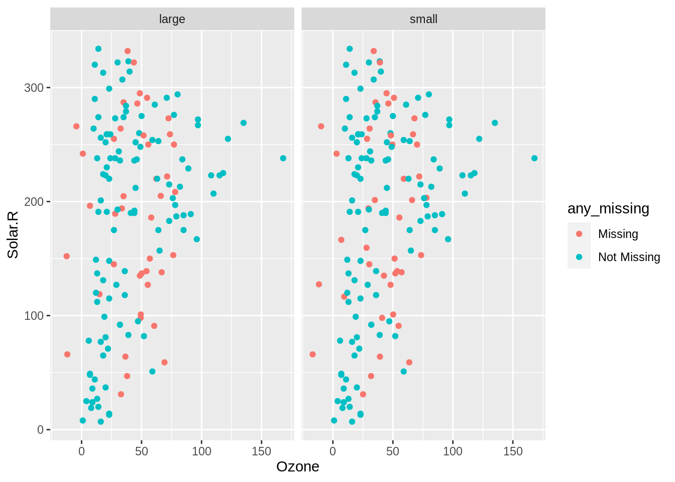
We can look at the values of Ozone and Solar.R on a scatterplot, colouring by any missings, and facetting by imputation model used: imp_model.

ggplot(bound_models,
       aes(x = Ozone,
           y = Solar.R,
           colour = any_missing)) +
  geom_point() + 
  facet_wrap(~imp_model)

We learn there isn’t much difference between either of the linear model methods for imputing data - they both seem to be within the range of the data, but both models did not impute three values.

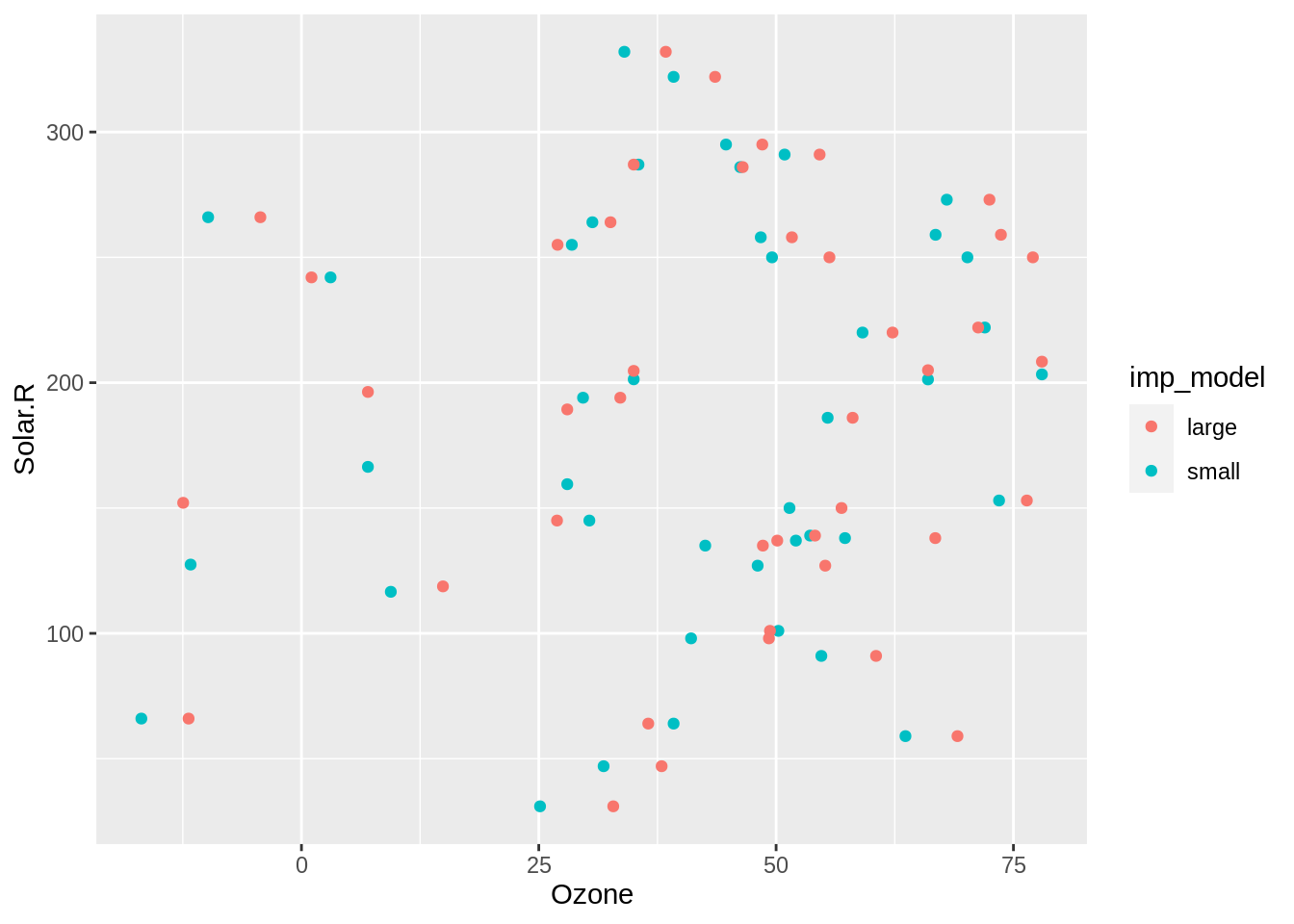
We can explore only the imputed values against each other by filtering to just “missing” (imputed) values, then plotting them, colouring by the different imputation model.

bound_models %>% 
  filter(any_missing == "Missing") %>% 
  ggplot(aes(x = Ozone,
             y = Solar.R,
             colour = imp_model)) +
  geom_point()

We learn that there appears to be some difference in the imputed values, with perhaps the large imputation model imputing higher ozone levels than the small imputation model. We’ll go into a bit more detail on comparing between variable4s in the next section.

14.5 Explore imputations in multiple variables and models

To explore the imputations across these different models and variables, we gather the selected four variables, Ozone, Solar Radiation, any_missing, and imp_model, and then we pivot the Ozone and Solar.R variables into longer form with pivot_longer().

bound_models_gather <- bound_models %>%
  select(Ozone, 
         Solar.R,
         any_missing, 
         imp_model) %>%
  pivot_longer(cols = c(Ozone, Solar.R),
               names_to = "variable",
               values_to = "value")

bound_models_gather

# A tibble: 612 × 4
   any_missing imp_model variable value
   <chr>       <chr>     <chr>    <dbl>
 1 Not Missing small     Ozone     41  
 2 Not Missing small     Solar.R  190  
 3 Not Missing small     Ozone     36  
 4 Not Missing small     Solar.R  118  
 5 Not Missing small     Ozone     12  
 6 Not Missing small     Solar.R  149  
 7 Not Missing small     Ozone     18  
 8 Not Missing small     Solar.R  313  
 9 Missing     small     Ozone    -11.7
10 Missing     small     Solar.R  127. 
# … with 602 more rows

This gives us the columns, any_missing, imp_model, variable, and value:

head(bound_models_gather)

# A tibble: 6 × 4
  any_missing imp_model variable value
  <chr>       <chr>     <chr>    <dbl>
1 Not Missing small     Ozone       41
2 Not Missing small     Solar.R    190
3 Not Missing small     Ozone       36
4 Not Missing small     Solar.R    118
5 Not Missing small     Ozone       12
6 Not Missing small     Solar.R    149

tail(bound_models_gather)

# A tibble: 6 × 4
  any_missing imp_model variable value
  <chr>       <chr>     <chr>    <dbl>
1 Not Missing large     Ozone       14
2 Not Missing large     Solar.R    191
3 Not Missing large     Ozone       18
4 Not Missing large     Solar.R    131
5 Not Missing large     Ozone       20
6 Not Missing large     Solar.R    223

14.5.1 Explore imputations in multiple variables and models

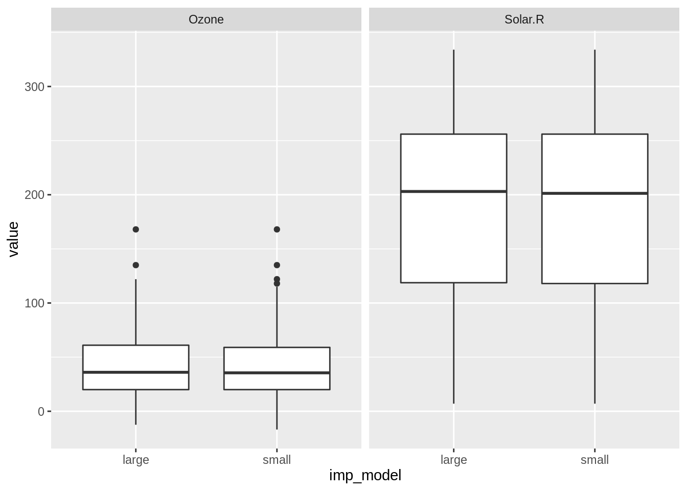
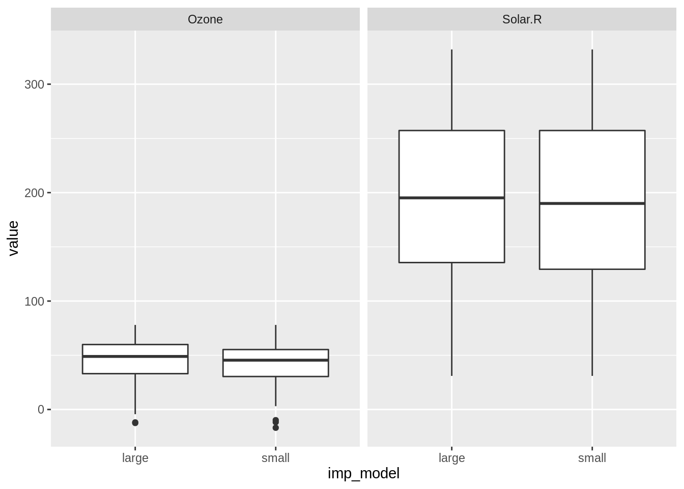
We can then plot the data as a boxplot, putting the imputation model on the x axis, value on the y axis, and facetting the different values for each variable.

ggplot(bound_models_gather,
       aes(x = imp_model,
           y = value)) +
  geom_boxplot() + 
  facet_wrap(~variable)

We learn that both models have similar mean and spread, and scale - there isn’t much difference between the models.

14.6 Explore imputations in multiple variables and models

We can also only look at the imputed values only, by filtering any_missing to look at “Missing”, and do the same plot.

bound_models_gather %>%
  filter(any_missing == "Missing") %>%
  ggplot(aes(x = imp_model,
             y = value)) +
  geom_boxplot() + 
  facet_wrap(~variable)

We see that the imputed values for the larger model tend to have a slightly higher median than those imputed with the smaller model. But this is a very small difference.