8 Representing Missing Data
This book contains both practical guides on exploring missing data, as well as some of the deeper details of how naniar works to help you better explore your missing data. A large component of this book are the exercises that accompany each section in each chapter.
We’ve covered how to create summaries and visualize missing values. But how do we link these summaries of missingness back to values in the data? This chapter explores two special data structures to facilitate working with missing data:
- The Shadow Matrix
- Nabular data
8.1 Motivation
Let’s imagine that we have some census data that contains two columns: income, and education.
Rows: 200 Columns: 2
── Column specification ────────────────────────────────────────────────────────
Delimiter: ","
chr (1): education
dbl (1): income

ℹ Use `spec()` to retrieve the full column specification for this data.
ℹ Specify the column types or set `show_col_types = FALSE` to quiet this message.| income | education |
|---|---|
| 73.13497 | NA |
| 66.78344 | high_school |
| 47.18483 | NA |
| 31.19808 | high_school |
| 64.41645 | NA |
| 51.80495 | NA |
There are some missing values in education. If we look at the distribution of income, we see that it looks like most of the values are around 70-80 thousand dollars a year.
ggplot(census,
       aes(x = income)) +
  geom_density()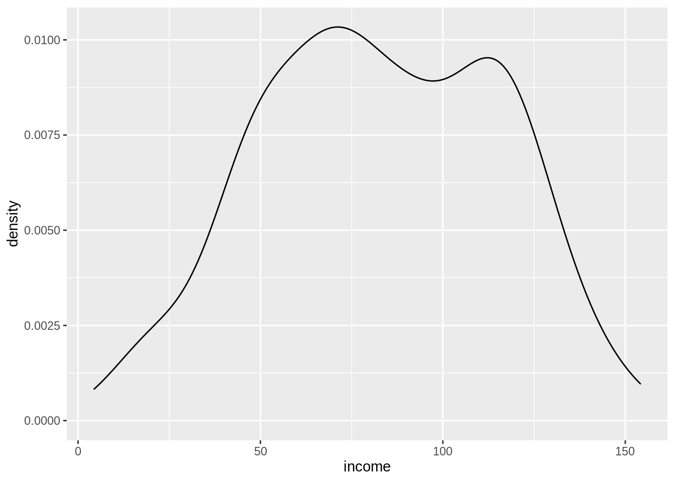
But if we create a new variable that tells us if education is missing, education_NA, using if_else. This will contain the value “NA” when education is missing, and “!NA” when education is not missing (! meaning NOT).
census_na <- census %>%
  mutate(education_NA = if_else(condition = is.na(education),
                                true = "NA",
                                false = "!NA"))

census_na
# A tibble: 200 × 3
income education education_NA
<dbl> <chr> <chr>
1 73.1 <NA> NA
2 66.8 high_school !NA
3 47.2 <NA> NA
4 31.2 high_school !NA
5 64.4 <NA> NA
6 51.8 <NA> NA
7 52.6 <NA> NA
8 17.5 high_school !NA
9 61.2 <NA> NA
10 21.2 high_school !NA
# … with 190 more rowsThen this new variable education_NA allows us to explore how income changes depending on whether or not education is missing.
ggplot(census_na,
       aes(x = income,
           fill = education_NA)) +
  geom_density(alpha = 0.5)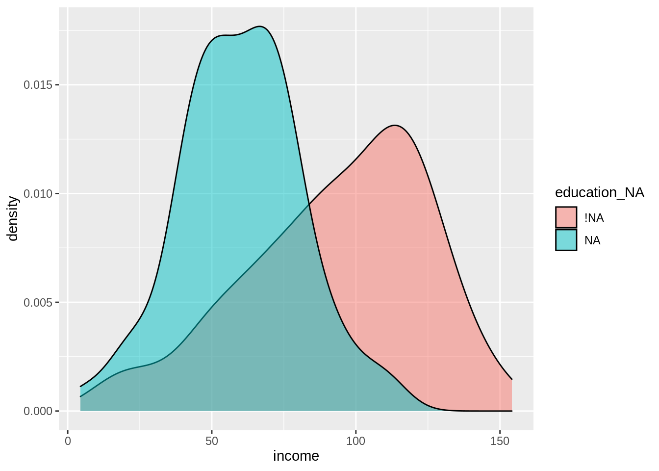
We can see that indeed, your value of income does change whether your education value is missing or not.
Plots like this are really useful to explore missingness in a more principled way. naniar provides special data structures that facilitate this in a powerful way. This chapter introduces these special data structures, the shadow matrix, and nabular data, and demonstrates how their use in analysis.
8.2 The shadow matrix
We previously showed how the new variable, education_NA can be used to explore missing data. This variable can be thought of as the “shadow” of education:
census_na %>%
  select(education,
         education_NA) %>%
  slice(1:10) %>%
knitr::kable()| education | education_NA |
|---|---|
| NA | NA |
| high_school | !NA |
| NA | NA |
| high_school | !NA |
| NA | NA |
| NA | NA |
| NA | NA |
| high_school | !NA |
| NA | NA |
| high_school | !NA |
Creating these shadow variables is handy! But doing it for each variable, each time you want to explore missingness adds a lot of extra work. We can instead shift our focus to look at what if we turned all of the variables into shadow versions of themselves. We call this a “Shadow matrix”. You can convert your data to a shadow matrix using as_shadow().
as_shadow(census)# A tibble: 200 × 2
income_NA education_NA
<fct> <fct>
1 !NA NA
2 !NA !NA
3 !NA NA
4 !NA !NA
5 !NA NA
6 !NA NA
7 !NA NA
8 !NA !NA
9 !NA NA
10 !NA !NA
# … with 190 more rowsWhile you can get something similar by using is.na()
is.na(census) %>% head() income education
[1,] FALSE TRUE
[2,] FALSE FALSE
[3,] FALSE TRUE
[4,] FALSE FALSE
[5,] FALSE TRUE
[6,] FALSE TRUEThis is has some shortcomings - the first being that it is now actually a matrix, not a dataframe:
is.na(census) %>% head() %>% class()[1] "matrix" "array" and the second being that it is not entirely clear what TRUE means! Does it mean TRUE missing or TRUE, present? The shadow matrix from as_shadow returns a dataframe, and contains two features that make it easier to use in a data analysis:
Coordinated names: Variables in the shadow matrix gain the same name as in the data, with the suffix “_NA”. This makes the variables missingness clear to refer to. It also indicates that we shift our thinking from “what is this variable’s values” to “what is the missingness of this variable”.
Clear values. The values are either !NA - “not missing”, or NA - “missing”. This is clearer than 1s and 0s for missing/not missing
The shadow matrix is most useful when combined with the data, which we call nabular data, which we now discuss.
8.3 Creating nabular data
To get the most out of the shadow matrix, it needs to be attached, column-wise, to the data. Putting the data in this form is referred to as nabular data - so called because it is a portmanteau or “NA”, and “Tabular”. You can create this data with nabular():
nabular(census)# A tibble: 200 × 4
income education income_NA education_NA
<dbl> <chr> <fct> <fct>
1 73.1 <NA> !NA NA
2 66.8 high_school !NA !NA
3 47.2 <NA> !NA NA
4 31.2 high_school !NA !NA
5 64.4 <NA> !NA NA
6 51.8 <NA> !NA NA
7 52.6 <NA> !NA NA
8 17.5 high_school !NA !NA
9 61.2 <NA> !NA NA
10 21.2 high_school !NA !NA
# … with 190 more rowsSo here we have the income values and education, and then their shadow representations - income_NA, and education_NA.
An aside: data storage and nabular data
It’s worth mentioning that using nabular data does increase the size of your data:
lobstr::obj_size(census)6.38 kBlobstr::obj_size(nabular(census))7.70 kBlobstr::obj_size(riskfactors)49.23 kBlobstr::obj_size(nabular(riskfactors))99.99 kBif size is an issue for you, one option could be to down sample your data. The philosophy behind exploring your data with naniar is to get a handle on the general issues of missing data first. Although speed is important, we want to make sure that these techniques work well before making them super fast. In the future we will hopefully explore some techniques for making the size of
nabulardata smaller.
One way to reduce
nabulardata size is to only addshadowcolumns for values that are missing, using theonly_missargument innabular:
lobstr::obj_size(riskfactors)49.23 kBlobstr::obj_size(nabular(riskfactors))99.99 kBnabular(riskfactors, only_miss = TRUE)# A tibble: 245 × 58
state sex age weight_lbs height_inch bmi marital pregnant children
<fct> <fct> <int> <int> <int> <dbl> <fct> <fct> <int>
1 26 Female 49 190 64 32.7 Married <NA> 0
2 40 Female 48 170 68 25.9 Divorced <NA> 0
3 72 Female 55 163 64 28.0 Married <NA> 0
4 42 Male 42 230 74 29.6 Married <NA> 1
5 32 Female 66 135 62 24.7 Widowed <NA> 0
6 19 Male 66 165 70 23.7 Married <NA> 0
7 45 Male 37 150 68 22.9 Married <NA> 3
8 56 Female 62 170 70 24.4 NeverMarri… <NA> 0
9 18 Male 38 146 70 21.0 Married <NA> 2
10 8 Female 42 260 73 34.4 Separated No 3
# … with 235 more rows, and 49 more variables: education <fct>,
# employment <fct>, income <fct>, veteran <fct>, hispanic <fct>,
# health_general <fct>, health_physical <int>, health_mental <int>,
# health_poor <int>, health_cover <fct>, provide_care <fct>,
# activity_limited <fct>, drink_any <fct>, drink_days <int>,
# drink_average <int>, smoke_100 <fct>, smoke_days <fct>, smoke_stop <fct>,
# smoke_last <fct>, diet_fruit <int>, diet_salad <int>, diet_potato <int>, …lobstr::obj_size(nabular(riskfactors, only_miss = TRUE))85.24 kB8.4 Data summaries with nabular data
Now that you can create nabular data, let’s use it to do something useful, like calculate summary statistics based on the missingness of something else. We take the airquality data, then use nabular() to turn the data into nabular data.
nabular(airquality)# A tibble: 153 × 12
Ozone Solar.R Wind Temp Month Day Ozone_NA Solar.R_NA Wind_NA Temp_NA
<int> <int> <dbl> <int> <int> <int> <fct> <fct> <fct> <fct>
1 41 190 7.4 67 5 1 !NA !NA !NA !NA
2 36 118 8 72 5 2 !NA !NA !NA !NA
3 12 149 12.6 74 5 3 !NA !NA !NA !NA
4 18 313 11.5 62 5 4 !NA !NA !NA !NA
5 NA NA 14.3 56 5 5 NA NA !NA !NA
6 28 NA 14.9 66 5 6 !NA NA !NA !NA
7 23 299 8.6 65 5 7 !NA !NA !NA !NA
8 19 99 13.8 59 5 8 !NA !NA !NA !NA
9 8 19 20.1 61 5 9 !NA !NA !NA !NA
10 NA 194 8.6 69 5 10 NA !NA !NA !NA
# … with 143 more rows, and 2 more variables: Month_NA <fct>, Day_NA <fct>Note that we have the airquality variables, Ozone, Solar.R, etc., and the shadow matrix variables, Ozone_NA, Solar.R_NA and so on.
We can perform some summaries on the data using group_by and summarise() to calculate the mean of Wind speed, according to the missingness of Ozone:
airquality %>%
  nabular() %>%
  group_by(Ozone_NA) %>%
  summarise(mean = mean(Wind))
# A tibble: 2 × 2
Ozone_NA mean
<fct> <dbl>
1 !NA 9.86
2 NA 10.3 We see that the mean values of Wind are relatively similar, but slightly higher when Ozone is missing, than when Ozone is not missing.