In this section, we are going to focus on two areas:
Using imputations to understand data structure Visualising and exploring imputed values .
The goal is to develop skills in imputing data and tracking missing values, and visualising imputed values against data.
Some of these techniques might look familiar. This is one of the benefits to using naniar; the methods applied for exploring missing values are similar to exploring imputations.
Using imputations to understand data structure
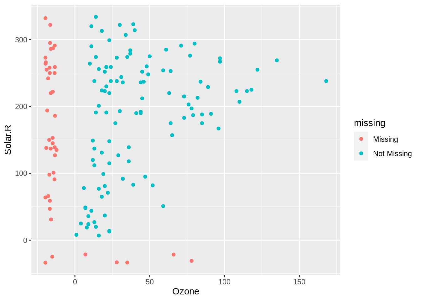
Previous chapters used geom_miss_point() to explore missing values. This “shifted” the missing values below the range of the data so we could see them.
ggplot (airquality,aes (x = Ozone,y = Solar.R)) + geom_miss_point ()
This shifting was actually “imputing” the data! Remember, “Impute” means to fill in a missing value. We are going to recreate these visualisations using impute_below() from naniar. This imputes values below the range of the data. For example, for this vector of numbers 5:10 with one missing value:
<- c (5 ,6 ,7 ,NA ,9 ,10 )impute_below (vec)
[1] 5.00000 6.00000 7.00000 4.40271 9.00000 10.00000
it imputes the value 4.4 into the missing value, since this is lower than the lowest value of the data at hand, namely 5.000.
impute_below()
We can use impute_below() in combination with mutate() to impute specific values.
For example:
%>% mutate (Ozone = impute_below (Ozone))
        Ozone Solar.R Wind Temp Month Day
1    41.00000     190  7.4   67     5   1
2    36.00000     118  8.0   72     5   2
3    12.00000     149 12.6   74     5   3
4    18.00000     313 11.5   62     5   4
5   -19.72321      NA 14.3   56     5   5
6    28.00000      NA 14.9   66     5   6
7    23.00000     299  8.6   65     5   7
8    19.00000      99 13.8   59     5   8
9     8.00000      19 20.1   61     5   9
10  -18.51277     194  8.6   69     5  10
11    7.00000      NA  6.9   74     5  11
12   16.00000     256  9.7   69     5  12
13   11.00000     290  9.2   66     5  13
14   14.00000     274 10.9   68     5  14
15   18.00000      65 13.2   58     5  15
16   14.00000     334 11.5   64     5  16
17   34.00000     307 12.0   66     5  17
18    6.00000      78 18.4   57     5  18
19   30.00000     322 11.5   68     5  19
20   11.00000      44  9.7   62     5  20
21    1.00000       8  9.7   59     5  21
22   11.00000     320 16.6   73     5  22
23    4.00000      25  9.7   61     5  23
24   32.00000      92 12.0   61     5  24
25  -17.81863      66 16.6   57     5  25
26  -19.43853     266 14.9   58     5  26
27  -15.14310      NA  8.0   57     5  27
28   23.00000      13 12.0   67     5  28
29   45.00000     252 14.9   81     5  29
30  115.00000     223  5.7   79     5  30
31   37.00000     279  7.4   76     5  31
32  -16.17315     286  8.6   78     6   1
33  -14.65883     287  9.7   74     6   2
34  -17.85609     242 16.1   67     6   3
35  -13.29299     186  9.2   84     6   4
36  -16.16323     220  8.6   85     6   5
37  -19.60935     264 14.3   79     6   6
38   29.00000     127  9.7   82     6   7
39  -19.65780     273  6.9   87     6   8
40   71.00000     291 13.8   90     6   9
41   39.00000     323 11.5   87     6  10
42  -13.40961     259 10.9   93     6  11
43  -13.53728     250  9.2   92     6  12
44   23.00000     148  8.0   82     6  13
45  -19.65993     332 13.8   80     6  14
46  -16.48342     322 11.5   79     6  15
47   21.00000     191 14.9   77     6  16
48   37.00000     284 20.7   72     6  17
49   20.00000      37  9.2   65     6  18
50   12.00000     120 11.5   73     6  19
51   13.00000     137 10.3   76     6  20
52  -17.17718     150  6.3   77     6  21
53  -16.74073      59  1.7   76     6  22
54  -13.65786      91  4.6   76     6  23
55  -16.78786     250  6.3   76     6  24
56  -12.30098     135  8.0   75     6  25
57  -13.33171     127  8.0   78     6  26
58  -16.77414      47 10.3   73     6  27
59  -17.08225      98 11.5   80     6  28
60  -15.98818      31 14.9   77     6  29
61  -19.17558     138  8.0   83     6  30
62  135.00000     269  4.1   84     7   1
63   49.00000     248  9.2   85     7   2
64   32.00000     236  9.2   81     7   3
65  -14.27138     101 10.9   84     7   4
66   64.00000     175  4.6   83     7   5
67   40.00000     314 10.9   83     7   6
68   77.00000     276  5.1   88     7   7
69   97.00000     267  6.3   92     7   8
70   97.00000     272  5.7   92     7   9
71   85.00000     175  7.4   89     7  10
72  -13.51764     139  8.6   82     7  11
73   10.00000     264 14.3   73     7  12
74   27.00000     175 14.9   81     7  13
75  -13.48998     291 14.9   91     7  14
76    7.00000      48 14.3   80     7  15
77   48.00000     260  6.9   81     7  16
78   35.00000     274 10.3   82     7  17
79   61.00000     285  6.3   84     7  18
80   79.00000     187  5.1   87     7  19
81   63.00000     220 11.5   85     7  20
82   16.00000       7  6.9   74     7  21
83  -16.92150     258  9.7   81     7  22
84  -16.60335     295 11.5   82     7  23
85   80.00000     294  8.6   86     7  24
86  108.00000     223  8.0   85     7  25
87   20.00000      81  8.6   82     7  26
88   52.00000      82 12.0   86     7  27
89   82.00000     213  7.4   88     7  28
90   50.00000     275  7.4   86     7  29
91   64.00000     253  7.4   83     7  30
92   59.00000     254  9.2   81     7  31
93   39.00000      83  6.9   81     8   1
94    9.00000      24 13.8   81     8   2
95   16.00000      77  7.4   82     8   3
96   78.00000      NA  6.9   86     8   4
97   35.00000      NA  7.4   85     8   5
98   66.00000      NA  4.6   87     8   6
99  122.00000     255  4.0   89     8   7
100  89.00000     229 10.3   90     8   8
101 110.00000     207  8.0   90     8   9
102 -14.78907     222  8.6   92     8  10
103 -16.19151     137 11.5   86     8  11
104  44.00000     192 11.5   86     8  12
105  28.00000     273 11.5   82     8  13
106  65.00000     157  9.7   80     8  14
107 -19.73591      64 11.5   79     8  15
108  22.00000      71 10.3   77     8  16
109  59.00000      51  6.3   79     8  17
110  23.00000     115  7.4   76     8  18
111  31.00000     244 10.9   78     8  19
112  44.00000     190 10.3   78     8  20
113  21.00000     259 15.5   77     8  21
114   9.00000      36 14.3   72     8  22
115 -18.92235     255 12.6   75     8  23
116  45.00000     212  9.7   79     8  24
117 168.00000     238  3.4   81     8  25
118  73.00000     215  8.0   86     8  26
119 -14.86296     153  5.7   88     8  27
120  76.00000     203  9.7   97     8  28
121 118.00000     225  2.3   94     8  29
122  84.00000     237  6.3   96     8  30
123  85.00000     188  6.3   94     8  31
124  96.00000     167  6.9   91     9   1
125  78.00000     197  5.1   92     9   2
126  73.00000     183  2.8   93     9   3
127  91.00000     189  4.6   93     9   4
128  47.00000      95  7.4   87     9   5
129  32.00000      92 15.5   84     9   6
130  20.00000     252 10.9   80     9   7
131  23.00000     220 10.3   78     9   8
132  21.00000     230 10.9   75     9   9
133  24.00000     259  9.7   73     9  10
134  44.00000     236 14.9   81     9  11
135  21.00000     259 15.5   76     9  12
136  28.00000     238  6.3   77     9  13
137   9.00000      24 10.9   71     9  14
138  13.00000     112 11.5   71     9  15
139  46.00000     237  6.9   78     9  16
140  18.00000     224 13.8   67     9  17
141  13.00000      27 10.3   76     9  18
142  24.00000     238 10.3   68     9  19
143  16.00000     201  8.0   82     9  20
144  13.00000     238 12.6   64     9  21
145  23.00000      14  9.2   71     9  22
146  36.00000     139 10.3   81     9  23
147   7.00000      49 10.3   69     9  24
148  14.00000      20 16.6   63     9  25
149  30.00000     193  6.9   70     9  26
150 -14.83089     145 13.2   77     9  27
151  14.00000     191 14.3   75     9  28
152  18.00000     131  8.0   76     9  29
153  20.00000     223 11.5   68     9  30
However, sometimes you want to do this across many variables. Using the same approach for all variables in the dataset could be at best repetitive, and at worst lead to unintended mistakes. We can work around this by using across.
If we want to impute all variables, we can use across like so:
%>% mutate (across (everything (),impute_below))
        Ozone   Solar.R Wind Temp Month Day
1    41.00000 190.00000  7.4   67     5   1
2    36.00000 118.00000  8.0   72     5   2
3    12.00000 149.00000 12.6   74     5   3
4    18.00000 313.00000 11.5   62     5   4
5   -19.72321 -33.57778 14.3   56     5   5
6    28.00000 -33.07810 14.9   66     5   6
7    23.00000 299.00000  8.6   65     5   7
8    19.00000  99.00000 13.8   59     5   8
9     8.00000  19.00000 20.1   61     5   9
10  -18.51277 194.00000  8.6   69     5  10
11    7.00000 -21.37719  6.9   74     5  11
12   16.00000 256.00000  9.7   69     5  12
13   11.00000 290.00000  9.2   66     5  13
14   14.00000 274.00000 10.9   68     5  14
15   18.00000  65.00000 13.2   58     5  15
16   14.00000 334.00000 11.5   64     5  16
17   34.00000 307.00000 12.0   66     5  17
18    6.00000  78.00000 18.4   57     5  18
19   30.00000 322.00000 11.5   68     5  19
20   11.00000  44.00000  9.7   62     5  20
21    1.00000   8.00000  9.7   59     5  21
22   11.00000 320.00000 16.6   73     5  22
23    4.00000  25.00000  9.7   61     5  23
24   32.00000  92.00000 12.0   61     5  24
25  -17.81863  66.00000 16.6   57     5  25
26  -19.43853 266.00000 14.9   58     5  26
27  -15.14310 -24.60954  8.0   57     5  27
28   23.00000  13.00000 12.0   67     5  28
29   45.00000 252.00000 14.9   81     5  29
30  115.00000 223.00000  5.7   79     5  30
31   37.00000 279.00000  7.4   76     5  31
32  -16.17315 286.00000  8.6   78     6   1
33  -14.65883 287.00000  9.7   74     6   2
34  -17.85609 242.00000 16.1   67     6   3
35  -13.29299 186.00000  9.2   84     6   4
36  -16.16323 220.00000  8.6   85     6   5
37  -19.60935 264.00000 14.3   79     6   6
38   29.00000 127.00000  9.7   82     6   7
39  -19.65780 273.00000  6.9   87     6   8
40   71.00000 291.00000 13.8   90     6   9
41   39.00000 323.00000 11.5   87     6  10
42  -13.40961 259.00000 10.9   93     6  11
43  -13.53728 250.00000  9.2   92     6  12
44   23.00000 148.00000  8.0   82     6  13
45  -19.65993 332.00000 13.8   80     6  14
46  -16.48342 322.00000 11.5   79     6  15
47   21.00000 191.00000 14.9   77     6  16
48   37.00000 284.00000 20.7   72     6  17
49   20.00000  37.00000  9.2   65     6  18
50   12.00000 120.00000 11.5   73     6  19
51   13.00000 137.00000 10.3   76     6  20
52  -17.17718 150.00000  6.3   77     6  21
53  -16.74073  59.00000  1.7   76     6  22
54  -13.65786  91.00000  4.6   76     6  23
55  -16.78786 250.00000  6.3   76     6  24
56  -12.30098 135.00000  8.0   75     6  25
57  -13.33171 127.00000  8.0   78     6  26
58  -16.77414  47.00000 10.3   73     6  27
59  -17.08225  98.00000 11.5   80     6  28
60  -15.98818  31.00000 14.9   77     6  29
61  -19.17558 138.00000  8.0   83     6  30
62  135.00000 269.00000  4.1   84     7   1
63   49.00000 248.00000  9.2   85     7   2
64   32.00000 236.00000  9.2   81     7   3
65  -14.27138 101.00000 10.9   84     7   4
66   64.00000 175.00000  4.6   83     7   5
67   40.00000 314.00000 10.9   83     7   6
68   77.00000 276.00000  5.1   88     7   7
69   97.00000 267.00000  6.3   92     7   8
70   97.00000 272.00000  5.7   92     7   9
71   85.00000 175.00000  7.4   89     7  10
72  -13.51764 139.00000  8.6   82     7  11
73   10.00000 264.00000 14.3   73     7  12
74   27.00000 175.00000 14.9   81     7  13
75  -13.48998 291.00000 14.9   91     7  14
76    7.00000  48.00000 14.3   80     7  15
77   48.00000 260.00000  6.9   81     7  16
78   35.00000 274.00000 10.3   82     7  17
79   61.00000 285.00000  6.3   84     7  18
80   79.00000 187.00000  5.1   87     7  19
81   63.00000 220.00000 11.5   85     7  20
82   16.00000   7.00000  6.9   74     7  21
83  -16.92150 258.00000  9.7   81     7  22
84  -16.60335 295.00000 11.5   82     7  23
85   80.00000 294.00000  8.6   86     7  24
86  108.00000 223.00000  8.0   85     7  25
87   20.00000  81.00000  8.6   82     7  26
88   52.00000  82.00000 12.0   86     7  27
89   82.00000 213.00000  7.4   88     7  28
90   50.00000 275.00000  7.4   86     7  29
91   64.00000 253.00000  7.4   83     7  30
92   59.00000 254.00000  9.2   81     7  31
93   39.00000  83.00000  6.9   81     8   1
94    9.00000  24.00000 13.8   81     8   2
95   16.00000  77.00000  7.4   82     8   3
96   78.00000 -30.94374  6.9   86     8   4
97   35.00000 -33.38707  7.4   85     8   5
98   66.00000 -21.48980  4.6   87     8   6
99  122.00000 255.00000  4.0   89     8   7
100  89.00000 229.00000 10.3   90     8   8
101 110.00000 207.00000  8.0   90     8   9
102 -14.78907 222.00000  8.6   92     8  10
103 -16.19151 137.00000 11.5   86     8  11
104  44.00000 192.00000 11.5   86     8  12
105  28.00000 273.00000 11.5   82     8  13
106  65.00000 157.00000  9.7   80     8  14
107 -19.73591  64.00000 11.5   79     8  15
108  22.00000  71.00000 10.3   77     8  16
109  59.00000  51.00000  6.3   79     8  17
110  23.00000 115.00000  7.4   76     8  18
111  31.00000 244.00000 10.9   78     8  19
112  44.00000 190.00000 10.3   78     8  20
113  21.00000 259.00000 15.5   77     8  21
114   9.00000  36.00000 14.3   72     8  22
115 -18.92235 255.00000 12.6   75     8  23
116  45.00000 212.00000  9.7   79     8  24
117 168.00000 238.00000  3.4   81     8  25
118  73.00000 215.00000  8.0   86     8  26
119 -14.86296 153.00000  5.7   88     8  27
120  76.00000 203.00000  9.7   97     8  28
121 118.00000 225.00000  2.3   94     8  29
122  84.00000 237.00000  6.3   96     8  30
123  85.00000 188.00000  6.3   94     8  31
124  96.00000 167.00000  6.9   91     9   1
125  78.00000 197.00000  5.1   92     9   2
126  73.00000 183.00000  2.8   93     9   3
127  91.00000 189.00000  4.6   93     9   4
128  47.00000  95.00000  7.4   87     9   5
129  32.00000  92.00000 15.5   84     9   6
130  20.00000 252.00000 10.9   80     9   7
131  23.00000 220.00000 10.3   78     9   8
132  21.00000 230.00000 10.9   75     9   9
133  24.00000 259.00000  9.7   73     9  10
134  44.00000 236.00000 14.9   81     9  11
135  21.00000 259.00000 15.5   76     9  12
136  28.00000 238.00000  6.3   77     9  13
137   9.00000  24.00000 10.9   71     9  14
138  13.00000 112.00000 11.5   71     9  15
139  46.00000 237.00000  6.9   78     9  16
140  18.00000 224.00000 13.8   67     9  17
141  13.00000  27.00000 10.3   76     9  18
142  24.00000 238.00000 10.3   68     9  19
143  16.00000 201.00000  8.0   82     9  20
144  13.00000 238.00000 12.6   64     9  21
145  23.00000  14.00000  9.2   71     9  22
146  36.00000 139.00000 10.3   81     9  23
147   7.00000  49.00000 10.3   69     9  24
148  14.00000  20.00000 16.6   63     9  25
149  30.00000 193.00000  6.9   70     9  26
150 -14.83089 145.00000 13.2   77     9  27
151  14.00000 191.00000 14.3   75     9  28
152  18.00000 131.00000  8.0   76     9  29
153  20.00000 223.00000 11.5   68     9  30
Here we use the everything() helper function from dplyr, to select all variables. We can use any type of selection, from dplyrs tidy select
We can impute only those variables that satisfy a condition, like is this column numeric with is.numeric() using where() like so:
%>% mutate (across (where (is.numeric),impute_below))
        Ozone   Solar.R Wind Temp Month Day
1    41.00000 190.00000  7.4   67     5   1
2    36.00000 118.00000  8.0   72     5   2
3    12.00000 149.00000 12.6   74     5   3
4    18.00000 313.00000 11.5   62     5   4
5   -19.72321 -33.57778 14.3   56     5   5
6    28.00000 -33.07810 14.9   66     5   6
7    23.00000 299.00000  8.6   65     5   7
8    19.00000  99.00000 13.8   59     5   8
9     8.00000  19.00000 20.1   61     5   9
10  -18.51277 194.00000  8.6   69     5  10
11    7.00000 -21.37719  6.9   74     5  11
12   16.00000 256.00000  9.7   69     5  12
13   11.00000 290.00000  9.2   66     5  13
14   14.00000 274.00000 10.9   68     5  14
15   18.00000  65.00000 13.2   58     5  15
16   14.00000 334.00000 11.5   64     5  16
17   34.00000 307.00000 12.0   66     5  17
18    6.00000  78.00000 18.4   57     5  18
19   30.00000 322.00000 11.5   68     5  19
20   11.00000  44.00000  9.7   62     5  20
21    1.00000   8.00000  9.7   59     5  21
22   11.00000 320.00000 16.6   73     5  22
23    4.00000  25.00000  9.7   61     5  23
24   32.00000  92.00000 12.0   61     5  24
25  -17.81863  66.00000 16.6   57     5  25
26  -19.43853 266.00000 14.9   58     5  26
27  -15.14310 -24.60954  8.0   57     5  27
28   23.00000  13.00000 12.0   67     5  28
29   45.00000 252.00000 14.9   81     5  29
30  115.00000 223.00000  5.7   79     5  30
31   37.00000 279.00000  7.4   76     5  31
32  -16.17315 286.00000  8.6   78     6   1
33  -14.65883 287.00000  9.7   74     6   2
34  -17.85609 242.00000 16.1   67     6   3
35  -13.29299 186.00000  9.2   84     6   4
36  -16.16323 220.00000  8.6   85     6   5
37  -19.60935 264.00000 14.3   79     6   6
38   29.00000 127.00000  9.7   82     6   7
39  -19.65780 273.00000  6.9   87     6   8
40   71.00000 291.00000 13.8   90     6   9
41   39.00000 323.00000 11.5   87     6  10
42  -13.40961 259.00000 10.9   93     6  11
43  -13.53728 250.00000  9.2   92     6  12
44   23.00000 148.00000  8.0   82     6  13
45  -19.65993 332.00000 13.8   80     6  14
46  -16.48342 322.00000 11.5   79     6  15
47   21.00000 191.00000 14.9   77     6  16
48   37.00000 284.00000 20.7   72     6  17
49   20.00000  37.00000  9.2   65     6  18
50   12.00000 120.00000 11.5   73     6  19
51   13.00000 137.00000 10.3   76     6  20
52  -17.17718 150.00000  6.3   77     6  21
53  -16.74073  59.00000  1.7   76     6  22
54  -13.65786  91.00000  4.6   76     6  23
55  -16.78786 250.00000  6.3   76     6  24
56  -12.30098 135.00000  8.0   75     6  25
57  -13.33171 127.00000  8.0   78     6  26
58  -16.77414  47.00000 10.3   73     6  27
59  -17.08225  98.00000 11.5   80     6  28
60  -15.98818  31.00000 14.9   77     6  29
61  -19.17558 138.00000  8.0   83     6  30
62  135.00000 269.00000  4.1   84     7   1
63   49.00000 248.00000  9.2   85     7   2
64   32.00000 236.00000  9.2   81     7   3
65  -14.27138 101.00000 10.9   84     7   4
66   64.00000 175.00000  4.6   83     7   5
67   40.00000 314.00000 10.9   83     7   6
68   77.00000 276.00000  5.1   88     7   7
69   97.00000 267.00000  6.3   92     7   8
70   97.00000 272.00000  5.7   92     7   9
71   85.00000 175.00000  7.4   89     7  10
72  -13.51764 139.00000  8.6   82     7  11
73   10.00000 264.00000 14.3   73     7  12
74   27.00000 175.00000 14.9   81     7  13
75  -13.48998 291.00000 14.9   91     7  14
76    7.00000  48.00000 14.3   80     7  15
77   48.00000 260.00000  6.9   81     7  16
78   35.00000 274.00000 10.3   82     7  17
79   61.00000 285.00000  6.3   84     7  18
80   79.00000 187.00000  5.1   87     7  19
81   63.00000 220.00000 11.5   85     7  20
82   16.00000   7.00000  6.9   74     7  21
83  -16.92150 258.00000  9.7   81     7  22
84  -16.60335 295.00000 11.5   82     7  23
85   80.00000 294.00000  8.6   86     7  24
86  108.00000 223.00000  8.0   85     7  25
87   20.00000  81.00000  8.6   82     7  26
88   52.00000  82.00000 12.0   86     7  27
89   82.00000 213.00000  7.4   88     7  28
90   50.00000 275.00000  7.4   86     7  29
91   64.00000 253.00000  7.4   83     7  30
92   59.00000 254.00000  9.2   81     7  31
93   39.00000  83.00000  6.9   81     8   1
94    9.00000  24.00000 13.8   81     8   2
95   16.00000  77.00000  7.4   82     8   3
96   78.00000 -30.94374  6.9   86     8   4
97   35.00000 -33.38707  7.4   85     8   5
98   66.00000 -21.48980  4.6   87     8   6
99  122.00000 255.00000  4.0   89     8   7
100  89.00000 229.00000 10.3   90     8   8
101 110.00000 207.00000  8.0   90     8   9
102 -14.78907 222.00000  8.6   92     8  10
103 -16.19151 137.00000 11.5   86     8  11
104  44.00000 192.00000 11.5   86     8  12
105  28.00000 273.00000 11.5   82     8  13
106  65.00000 157.00000  9.7   80     8  14
107 -19.73591  64.00000 11.5   79     8  15
108  22.00000  71.00000 10.3   77     8  16
109  59.00000  51.00000  6.3   79     8  17
110  23.00000 115.00000  7.4   76     8  18
111  31.00000 244.00000 10.9   78     8  19
112  44.00000 190.00000 10.3   78     8  20
113  21.00000 259.00000 15.5   77     8  21
114   9.00000  36.00000 14.3   72     8  22
115 -18.92235 255.00000 12.6   75     8  23
116  45.00000 212.00000  9.7   79     8  24
117 168.00000 238.00000  3.4   81     8  25
118  73.00000 215.00000  8.0   86     8  26
119 -14.86296 153.00000  5.7   88     8  27
120  76.00000 203.00000  9.7   97     8  28
121 118.00000 225.00000  2.3   94     8  29
122  84.00000 237.00000  6.3   96     8  30
123  85.00000 188.00000  6.3   94     8  31
124  96.00000 167.00000  6.9   91     9   1
125  78.00000 197.00000  5.1   92     9   2
126  73.00000 183.00000  2.8   93     9   3
127  91.00000 189.00000  4.6   93     9   4
128  47.00000  95.00000  7.4   87     9   5
129  32.00000  92.00000 15.5   84     9   6
130  20.00000 252.00000 10.9   80     9   7
131  23.00000 220.00000 10.3   78     9   8
132  21.00000 230.00000 10.9   75     9   9
133  24.00000 259.00000  9.7   73     9  10
134  44.00000 236.00000 14.9   81     9  11
135  21.00000 259.00000 15.5   76     9  12
136  28.00000 238.00000  6.3   77     9  13
137   9.00000  24.00000 10.9   71     9  14
138  13.00000 112.00000 11.5   71     9  15
139  46.00000 237.00000  6.9   78     9  16
140  18.00000 224.00000 13.8   67     9  17
141  13.00000  27.00000 10.3   76     9  18
142  24.00000 238.00000 10.3   68     9  19
143  16.00000 201.00000  8.0   82     9  20
144  13.00000 238.00000 12.6   64     9  21
145  23.00000  14.00000  9.2   71     9  22
146  36.00000 139.00000 10.3   81     9  23
147   7.00000  49.00000 10.3   69     9  24
148  14.00000  20.00000 16.6   63     9  25
149  30.00000 193.00000  6.9   70     9  26
150 -14.83089 145.00000 13.2   77     9  27
151  14.00000 191.00000 14.3   75     9  28
152  18.00000 131.00000  8.0   76     9  29
153  20.00000 223.00000 11.5   68     9  30
This reads as:
Use airquality then across variables where they are numeric, impute below
We can choose specific variables like so:
%>% mutate (across (c (Ozone, Solar.R),impute_below))
        Ozone   Solar.R Wind Temp Month Day
1    41.00000 190.00000  7.4   67     5   1
2    36.00000 118.00000  8.0   72     5   2
3    12.00000 149.00000 12.6   74     5   3
4    18.00000 313.00000 11.5   62     5   4
5   -19.72321 -33.57778 14.3   56     5   5
6    28.00000 -33.07810 14.9   66     5   6
7    23.00000 299.00000  8.6   65     5   7
8    19.00000  99.00000 13.8   59     5   8
9     8.00000  19.00000 20.1   61     5   9
10  -18.51277 194.00000  8.6   69     5  10
11    7.00000 -21.37719  6.9   74     5  11
12   16.00000 256.00000  9.7   69     5  12
13   11.00000 290.00000  9.2   66     5  13
14   14.00000 274.00000 10.9   68     5  14
15   18.00000  65.00000 13.2   58     5  15
16   14.00000 334.00000 11.5   64     5  16
17   34.00000 307.00000 12.0   66     5  17
18    6.00000  78.00000 18.4   57     5  18
19   30.00000 322.00000 11.5   68     5  19
20   11.00000  44.00000  9.7   62     5  20
21    1.00000   8.00000  9.7   59     5  21
22   11.00000 320.00000 16.6   73     5  22
23    4.00000  25.00000  9.7   61     5  23
24   32.00000  92.00000 12.0   61     5  24
25  -17.81863  66.00000 16.6   57     5  25
26  -19.43853 266.00000 14.9   58     5  26
27  -15.14310 -24.60954  8.0   57     5  27
28   23.00000  13.00000 12.0   67     5  28
29   45.00000 252.00000 14.9   81     5  29
30  115.00000 223.00000  5.7   79     5  30
31   37.00000 279.00000  7.4   76     5  31
32  -16.17315 286.00000  8.6   78     6   1
33  -14.65883 287.00000  9.7   74     6   2
34  -17.85609 242.00000 16.1   67     6   3
35  -13.29299 186.00000  9.2   84     6   4
36  -16.16323 220.00000  8.6   85     6   5
37  -19.60935 264.00000 14.3   79     6   6
38   29.00000 127.00000  9.7   82     6   7
39  -19.65780 273.00000  6.9   87     6   8
40   71.00000 291.00000 13.8   90     6   9
41   39.00000 323.00000 11.5   87     6  10
42  -13.40961 259.00000 10.9   93     6  11
43  -13.53728 250.00000  9.2   92     6  12
44   23.00000 148.00000  8.0   82     6  13
45  -19.65993 332.00000 13.8   80     6  14
46  -16.48342 322.00000 11.5   79     6  15
47   21.00000 191.00000 14.9   77     6  16
48   37.00000 284.00000 20.7   72     6  17
49   20.00000  37.00000  9.2   65     6  18
50   12.00000 120.00000 11.5   73     6  19
51   13.00000 137.00000 10.3   76     6  20
52  -17.17718 150.00000  6.3   77     6  21
53  -16.74073  59.00000  1.7   76     6  22
54  -13.65786  91.00000  4.6   76     6  23
55  -16.78786 250.00000  6.3   76     6  24
56  -12.30098 135.00000  8.0   75     6  25
57  -13.33171 127.00000  8.0   78     6  26
58  -16.77414  47.00000 10.3   73     6  27
59  -17.08225  98.00000 11.5   80     6  28
60  -15.98818  31.00000 14.9   77     6  29
61  -19.17558 138.00000  8.0   83     6  30
62  135.00000 269.00000  4.1   84     7   1
63   49.00000 248.00000  9.2   85     7   2
64   32.00000 236.00000  9.2   81     7   3
65  -14.27138 101.00000 10.9   84     7   4
66   64.00000 175.00000  4.6   83     7   5
67   40.00000 314.00000 10.9   83     7   6
68   77.00000 276.00000  5.1   88     7   7
69   97.00000 267.00000  6.3   92     7   8
70   97.00000 272.00000  5.7   92     7   9
71   85.00000 175.00000  7.4   89     7  10
72  -13.51764 139.00000  8.6   82     7  11
73   10.00000 264.00000 14.3   73     7  12
74   27.00000 175.00000 14.9   81     7  13
75  -13.48998 291.00000 14.9   91     7  14
76    7.00000  48.00000 14.3   80     7  15
77   48.00000 260.00000  6.9   81     7  16
78   35.00000 274.00000 10.3   82     7  17
79   61.00000 285.00000  6.3   84     7  18
80   79.00000 187.00000  5.1   87     7  19
81   63.00000 220.00000 11.5   85     7  20
82   16.00000   7.00000  6.9   74     7  21
83  -16.92150 258.00000  9.7   81     7  22
84  -16.60335 295.00000 11.5   82     7  23
85   80.00000 294.00000  8.6   86     7  24
86  108.00000 223.00000  8.0   85     7  25
87   20.00000  81.00000  8.6   82     7  26
88   52.00000  82.00000 12.0   86     7  27
89   82.00000 213.00000  7.4   88     7  28
90   50.00000 275.00000  7.4   86     7  29
91   64.00000 253.00000  7.4   83     7  30
92   59.00000 254.00000  9.2   81     7  31
93   39.00000  83.00000  6.9   81     8   1
94    9.00000  24.00000 13.8   81     8   2
95   16.00000  77.00000  7.4   82     8   3
96   78.00000 -30.94374  6.9   86     8   4
97   35.00000 -33.38707  7.4   85     8   5
98   66.00000 -21.48980  4.6   87     8   6
99  122.00000 255.00000  4.0   89     8   7
100  89.00000 229.00000 10.3   90     8   8
101 110.00000 207.00000  8.0   90     8   9
102 -14.78907 222.00000  8.6   92     8  10
103 -16.19151 137.00000 11.5   86     8  11
104  44.00000 192.00000 11.5   86     8  12
105  28.00000 273.00000 11.5   82     8  13
106  65.00000 157.00000  9.7   80     8  14
107 -19.73591  64.00000 11.5   79     8  15
108  22.00000  71.00000 10.3   77     8  16
109  59.00000  51.00000  6.3   79     8  17
110  23.00000 115.00000  7.4   76     8  18
111  31.00000 244.00000 10.9   78     8  19
112  44.00000 190.00000 10.3   78     8  20
113  21.00000 259.00000 15.5   77     8  21
114   9.00000  36.00000 14.3   72     8  22
115 -18.92235 255.00000 12.6   75     8  23
116  45.00000 212.00000  9.7   79     8  24
117 168.00000 238.00000  3.4   81     8  25
118  73.00000 215.00000  8.0   86     8  26
119 -14.86296 153.00000  5.7   88     8  27
120  76.00000 203.00000  9.7   97     8  28
121 118.00000 225.00000  2.3   94     8  29
122  84.00000 237.00000  6.3   96     8  30
123  85.00000 188.00000  6.3   94     8  31
124  96.00000 167.00000  6.9   91     9   1
125  78.00000 197.00000  5.1   92     9   2
126  73.00000 183.00000  2.8   93     9   3
127  91.00000 189.00000  4.6   93     9   4
128  47.00000  95.00000  7.4   87     9   5
129  32.00000  92.00000 15.5   84     9   6
130  20.00000 252.00000 10.9   80     9   7
131  23.00000 220.00000 10.3   78     9   8
132  21.00000 230.00000 10.9   75     9   9
133  24.00000 259.00000  9.7   73     9  10
134  44.00000 236.00000 14.9   81     9  11
135  21.00000 259.00000 15.5   76     9  12
136  28.00000 238.00000  6.3   77     9  13
137   9.00000  24.00000 10.9   71     9  14
138  13.00000 112.00000 11.5   71     9  15
139  46.00000 237.00000  6.9   78     9  16
140  18.00000 224.00000 13.8   67     9  17
141  13.00000  27.00000 10.3   76     9  18
142  24.00000 238.00000 10.3   68     9  19
143  16.00000 201.00000  8.0   82     9  20
144  13.00000 238.00000 12.6   64     9  21
145  23.00000  14.00000  9.2   71     9  22
146  36.00000 139.00000 10.3   81     9  23
147   7.00000  49.00000 10.3   69     9  24
148  14.00000  20.00000 16.6   63     9  25
149  30.00000 193.00000  6.9   70     9  26
150 -14.83089 145.00000 13.2   77     9  27
151  14.00000 191.00000 14.3   75     9  28
152  18.00000 131.00000  8.0   76     9  29
153  20.00000 223.00000 11.5   68     9  30
We can take advantage of selection helpers from dplyrs tidy select
%>% mutate (across (c (Ozone, Solar.R, starts_with ("T" )),impute_below))
        Ozone   Solar.R Wind Temp Month Day
1    41.00000 190.00000  7.4   67     5   1
2    36.00000 118.00000  8.0   72     5   2
3    12.00000 149.00000 12.6   74     5   3
4    18.00000 313.00000 11.5   62     5   4
5   -19.72321 -33.57778 14.3   56     5   5
6    28.00000 -33.07810 14.9   66     5   6
7    23.00000 299.00000  8.6   65     5   7
8    19.00000  99.00000 13.8   59     5   8
9     8.00000  19.00000 20.1   61     5   9
10  -18.51277 194.00000  8.6   69     5  10
11    7.00000 -21.37719  6.9   74     5  11
12   16.00000 256.00000  9.7   69     5  12
13   11.00000 290.00000  9.2   66     5  13
14   14.00000 274.00000 10.9   68     5  14
15   18.00000  65.00000 13.2   58     5  15
16   14.00000 334.00000 11.5   64     5  16
17   34.00000 307.00000 12.0   66     5  17
18    6.00000  78.00000 18.4   57     5  18
19   30.00000 322.00000 11.5   68     5  19
20   11.00000  44.00000  9.7   62     5  20
21    1.00000   8.00000  9.7   59     5  21
22   11.00000 320.00000 16.6   73     5  22
23    4.00000  25.00000  9.7   61     5  23
24   32.00000  92.00000 12.0   61     5  24
25  -17.81863  66.00000 16.6   57     5  25
26  -19.43853 266.00000 14.9   58     5  26
27  -15.14310 -24.60954  8.0   57     5  27
28   23.00000  13.00000 12.0   67     5  28
29   45.00000 252.00000 14.9   81     5  29
30  115.00000 223.00000  5.7   79     5  30
31   37.00000 279.00000  7.4   76     5  31
32  -16.17315 286.00000  8.6   78     6   1
33  -14.65883 287.00000  9.7   74     6   2
34  -17.85609 242.00000 16.1   67     6   3
35  -13.29299 186.00000  9.2   84     6   4
36  -16.16323 220.00000  8.6   85     6   5
37  -19.60935 264.00000 14.3   79     6   6
38   29.00000 127.00000  9.7   82     6   7
39  -19.65780 273.00000  6.9   87     6   8
40   71.00000 291.00000 13.8   90     6   9
41   39.00000 323.00000 11.5   87     6  10
42  -13.40961 259.00000 10.9   93     6  11
43  -13.53728 250.00000  9.2   92     6  12
44   23.00000 148.00000  8.0   82     6  13
45  -19.65993 332.00000 13.8   80     6  14
46  -16.48342 322.00000 11.5   79     6  15
47   21.00000 191.00000 14.9   77     6  16
48   37.00000 284.00000 20.7   72     6  17
49   20.00000  37.00000  9.2   65     6  18
50   12.00000 120.00000 11.5   73     6  19
51   13.00000 137.00000 10.3   76     6  20
52  -17.17718 150.00000  6.3   77     6  21
53  -16.74073  59.00000  1.7   76     6  22
54  -13.65786  91.00000  4.6   76     6  23
55  -16.78786 250.00000  6.3   76     6  24
56  -12.30098 135.00000  8.0   75     6  25
57  -13.33171 127.00000  8.0   78     6  26
58  -16.77414  47.00000 10.3   73     6  27
59  -17.08225  98.00000 11.5   80     6  28
60  -15.98818  31.00000 14.9   77     6  29
61  -19.17558 138.00000  8.0   83     6  30
62  135.00000 269.00000  4.1   84     7   1
63   49.00000 248.00000  9.2   85     7   2
64   32.00000 236.00000  9.2   81     7   3
65  -14.27138 101.00000 10.9   84     7   4
66   64.00000 175.00000  4.6   83     7   5
67   40.00000 314.00000 10.9   83     7   6
68   77.00000 276.00000  5.1   88     7   7
69   97.00000 267.00000  6.3   92     7   8
70   97.00000 272.00000  5.7   92     7   9
71   85.00000 175.00000  7.4   89     7  10
72  -13.51764 139.00000  8.6   82     7  11
73   10.00000 264.00000 14.3   73     7  12
74   27.00000 175.00000 14.9   81     7  13
75  -13.48998 291.00000 14.9   91     7  14
76    7.00000  48.00000 14.3   80     7  15
77   48.00000 260.00000  6.9   81     7  16
78   35.00000 274.00000 10.3   82     7  17
79   61.00000 285.00000  6.3   84     7  18
80   79.00000 187.00000  5.1   87     7  19
81   63.00000 220.00000 11.5   85     7  20
82   16.00000   7.00000  6.9   74     7  21
83  -16.92150 258.00000  9.7   81     7  22
84  -16.60335 295.00000 11.5   82     7  23
85   80.00000 294.00000  8.6   86     7  24
86  108.00000 223.00000  8.0   85     7  25
87   20.00000  81.00000  8.6   82     7  26
88   52.00000  82.00000 12.0   86     7  27
89   82.00000 213.00000  7.4   88     7  28
90   50.00000 275.00000  7.4   86     7  29
91   64.00000 253.00000  7.4   83     7  30
92   59.00000 254.00000  9.2   81     7  31
93   39.00000  83.00000  6.9   81     8   1
94    9.00000  24.00000 13.8   81     8   2
95   16.00000  77.00000  7.4   82     8   3
96   78.00000 -30.94374  6.9   86     8   4
97   35.00000 -33.38707  7.4   85     8   5
98   66.00000 -21.48980  4.6   87     8   6
99  122.00000 255.00000  4.0   89     8   7
100  89.00000 229.00000 10.3   90     8   8
101 110.00000 207.00000  8.0   90     8   9
102 -14.78907 222.00000  8.6   92     8  10
103 -16.19151 137.00000 11.5   86     8  11
104  44.00000 192.00000 11.5   86     8  12
105  28.00000 273.00000 11.5   82     8  13
106  65.00000 157.00000  9.7   80     8  14
107 -19.73591  64.00000 11.5   79     8  15
108  22.00000  71.00000 10.3   77     8  16
109  59.00000  51.00000  6.3   79     8  17
110  23.00000 115.00000  7.4   76     8  18
111  31.00000 244.00000 10.9   78     8  19
112  44.00000 190.00000 10.3   78     8  20
113  21.00000 259.00000 15.5   77     8  21
114   9.00000  36.00000 14.3   72     8  22
115 -18.92235 255.00000 12.6   75     8  23
116  45.00000 212.00000  9.7   79     8  24
117 168.00000 238.00000  3.4   81     8  25
118  73.00000 215.00000  8.0   86     8  26
119 -14.86296 153.00000  5.7   88     8  27
120  76.00000 203.00000  9.7   97     8  28
121 118.00000 225.00000  2.3   94     8  29
122  84.00000 237.00000  6.3   96     8  30
123  85.00000 188.00000  6.3   94     8  31
124  96.00000 167.00000  6.9   91     9   1
125  78.00000 197.00000  5.1   92     9   2
126  73.00000 183.00000  2.8   93     9   3
127  91.00000 189.00000  4.6   93     9   4
128  47.00000  95.00000  7.4   87     9   5
129  32.00000  92.00000 15.5   84     9   6
130  20.00000 252.00000 10.9   80     9   7
131  23.00000 220.00000 10.3   78     9   8
132  21.00000 230.00000 10.9   75     9   9
133  24.00000 259.00000  9.7   73     9  10
134  44.00000 236.00000 14.9   81     9  11
135  21.00000 259.00000 15.5   76     9  12
136  28.00000 238.00000  6.3   77     9  13
137   9.00000  24.00000 10.9   71     9  14
138  13.00000 112.00000 11.5   71     9  15
139  46.00000 237.00000  6.9   78     9  16
140  18.00000 224.00000 13.8   67     9  17
141  13.00000  27.00000 10.3   76     9  18
142  24.00000 238.00000 10.3   68     9  19
143  16.00000 201.00000  8.0   82     9  20
144  13.00000 238.00000 12.6   64     9  21
145  23.00000  14.00000  9.2   71     9  22
146  36.00000 139.00000 10.3   81     9  23
147   7.00000  49.00000 10.3   69     9  24
148  14.00000  20.00000 16.6   63     9  25
149  30.00000 193.00000  6.9   70     9  26
150 -14.83089 145.00000 13.2   77     9  27
151  14.00000 191.00000 14.3   75     9  28
152  18.00000 131.00000  8.0   76     9  29
153  20.00000 223.00000 11.5   68     9  30
Tracking missing values
We need to track the missing values, once we impute them. Otherwise we don’t know what was imputed and what was not. We can see that in this example, once we impute the data, we have no way to recognise which one it is.
<- tibble (var1 = c (5 , 6 , 7 , NA , 9 , 10 ))
# A tibble: 6 × 1
   var1
  <dbl>
1     5
2     6
3     7
4    NA
5     9
6    10
%>% mutate (across (everything (),impute_below))
# A tibble: 6 × 1
   var1
  <dbl>
1  5
2  6
3  7
4  4.40
5  9
6 10
We can identify missings by using nabular to turn the data into nabular form.
# A tibble: 6 × 2
   var1 var1_NA
  <dbl> <fct>
1     5 !NA
2     6 !NA
3     7 !NA
4    NA NA
5     9 !NA
6    10 !NA
Now when we impute the data, we can see that the shadow variable, var1_NA reveals the imputed value, 4.40.
%>% nabular () %>% mutate (across (everything (),impute_below))
# A tibble: 6 × 2
   var1 var1_NA
  <dbl> <fct>
1  5    !NA
2  6    !NA
3  7    !NA
4  4.40 NA
5  9    !NA
6 10    !NA
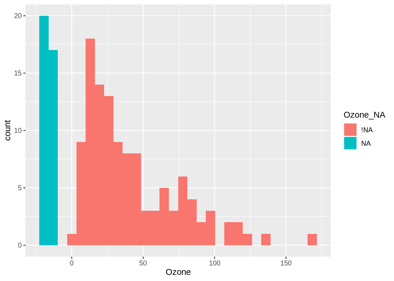
Visualise imputed values against data values using histograms
Using this imputed data, we can explore the number of missings in a single variable, along with it’s distribution, using a histogram and colouring the missings using fill = Ozone_NA.
<- airquality %>% nabular () %>% mutate (across (everything (),impute_below))ggplot (aq_imp,aes (x = Ozone,fill = Ozone_NA)) + geom_histogram ()
`stat_bin()` using `bins = 30`. Pick better value with `binwidth`.
Here we see that there are a few missing values - two bars around 20, so just under 40 missing values.
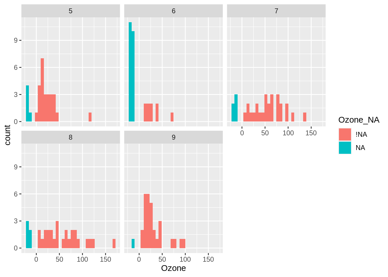
Visualise imputed values against data values using facets
We can take this same plot and visualise it across facets. For example, plot it by month, which shows us that most missing values occur in month 6 - which didn’t have many high values of ozone.
ggplot (aq_imp,aes (x = Ozone,fill = Ozone_NA)) + geom_histogram () + facet_wrap (~ Month)
`stat_bin()` using `bins = 30`. Pick better value with `binwidth`.
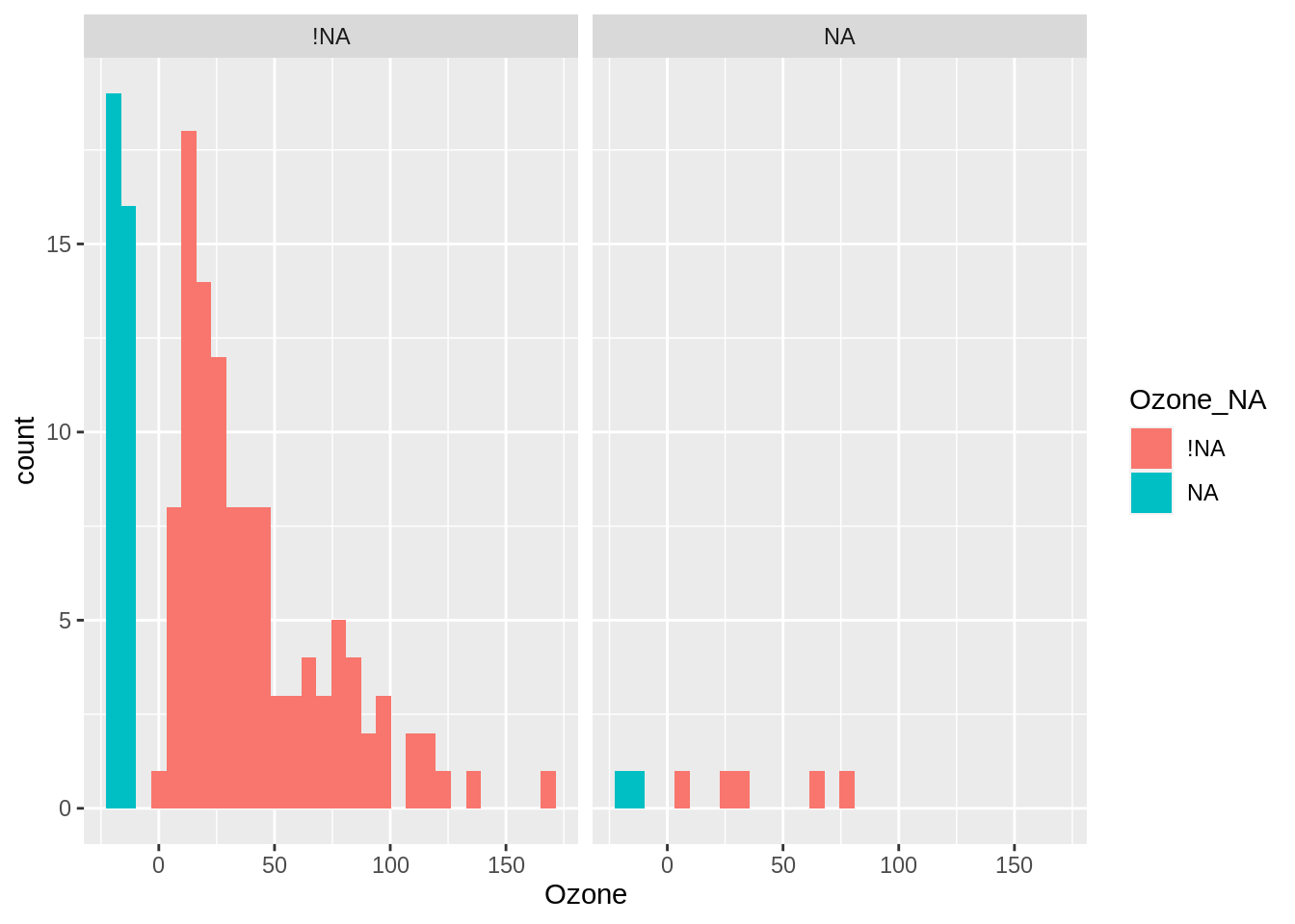
Visualize imputed values using facets
We can split the plot according to the missingness of solar radiation by referring to it as Solar.R_NA
ggplot (aq_imp,aes (x = Ozone,fill = Ozone_NA)) + geom_histogram () + facet_wrap (~ Solar.R_NA)
`stat_bin()` using `bins = 30`. Pick better value with `binwidth`.
This shows us that there aren’t many missing values in ozone when solar radiation is missing.
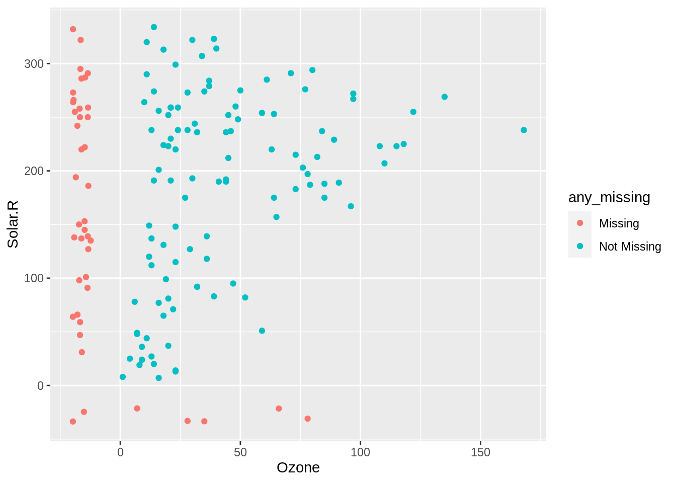
Visualize imputed values against data values using scatterplots
Previously we could identify imputed values by referring to the shadow variable - e.g., Ozone_NA. However, if you want to colour by two variables, you just need to know if any of them were imputed . We can add a column with labels to identify whether there is a missing value in a column. The function add_label_missings does this for us, adding a column, any_missing.
<- airquality %>% nabular () %>% add_label_missings () %>% mutate (across (everything (),impute_below))
# A tibble: 153 × 13
   Ozone Solar.R  Wind  Temp Month   Day Ozone_NA Solar.R_NA Wind_NA Temp_NA
   <dbl>   <dbl> <dbl> <int> <int> <int> <fct>    <fct>      <fct>   <fct>
 1  41     190     7.4    67     5     1 !NA      !NA        !NA     !NA
 2  36     118     8      72     5     2 !NA      !NA        !NA     !NA
 3  12     149    12.6    74     5     3 !NA      !NA        !NA     !NA
 4  18     313    11.5    62     5     4 !NA      !NA        !NA     !NA
 5 -19.7   -33.6  14.3    56     5     5 NA       NA         !NA     !NA
 6  28     -33.1  14.9    66     5     6 !NA      NA         !NA     !NA
 7  23     299     8.6    65     5     7 !NA      !NA        !NA     !NA
 8  19      99    13.8    59     5     8 !NA      !NA        !NA     !NA
 9   8      19    20.1    61     5     9 !NA      !NA        !NA     !NA
10 -18.5   194     8.6    69     5    10 NA       !NA        !NA     !NA
# … with 143 more rows, and 3 more variables: Month_NA <fct>, Day_NA <fct>,
#   any_missing <chr>
We can now recreate the same figure as geom_miss_point()!
ggplot (aq_imp,aes (x = Ozone,y = Solar.R,colour = any_missing)) + geom_point ()